Using Scoped Assignments To Show Calendar and Financial Year-To-Date Values In The Same Calculated Measure

I’ve had a lot of requests for more MDX content on my blog, so here’s something I’ve been meaning to write up for a long time: a worked example of how to use scoped assignments to implement two different types year-to-date calculation on two different hierarchies in the same dimension. Knowledge of how to use scoped assignments is the sign of a true MDX master (you can watch a video of a session I gave on the basics of scoped assignments at SQLBits here if you’re unfamiliar with them) but that’s because they can be very difficult to write and there’s surprisingly little information out there on the internet about them. They are incredibly powerful, though, and often they provide the most elegant and best-performing way to solve a problem.

Let’s start by looking at the Date dimension in the Adventure Works DW sample database, and more specifically the attributes, user hierarchies and attribute relationships:

image

image

Notice how we have two user hierarchies for Calendar Years (which start on January 1st) and Fiscal Years (which start on July 1st), called Calendar and Fiscal. Now, let’s say that you have a requirement to to show year-to-date values for a measure for both the Calendar and Fiscal hierarchies. It would be very easy to implement this as two separate calculated measures but what if you needed to show both types of year-to-date in the same calculated measure, showing Fiscal year-to-dates when the Fiscal hierarchy was used in a query and Calendar year-to-dates when the Calendar hierarchy was used in a query?

This is possible using scoped assignments. The first thing to point out, though, is that this is only going to be possible if you change the structure of the dimension. Why? Well, take a look at the Date levels of both hierarchies: they are both built using the Date attribute. If you were running a query with your YTD calculation on columns and only the Date attribute hierarchy on rows, would you expect to see Calendar or Fiscal YTD values? Certainly you couldn’t see both in the same cell, and this is the problem: if you expect to see Calendar YTD values at the bottom of your Calendar hierarchy, and Fiscal YTD values at the bottom of your Fiscal hierarchy, you need two separate Date attributes to do this. If you overwrite the values in the same cells twice using a scoped assignment, then you will only see the result of the second assignment.

Therefore, what we need to do is to create two new attributes, Calendar Date and Fiscal Date, to serve as the lowest levels of the Calendar and Fiscal hierarchies instead of the Date attribute. Here’s what the new attribute relationships look like:

image

From the end-user’s point of view nothing seems to have changed (these new attributes can have their AttributeHierarchyVisible property set to False) but this now means we have two attributes, two different slices of the cube, whose values we can overwrite separately instead of just one.

Now for the MDX. A good rule to follow when writing scoped assignments is to always use attribute hierarchies and never use user hierarchies; this is because there are rules you have to obey about the shape of the subcube of data you are overwriting with your scoped assignment. When defining a scope using only attribute hierarchies, you can only use the following types of set:

  • Every single member on the attribute hierarchy
  • Just one member on the attribute hierarchy
  • Multiple members on the attribute hierarchy not including the All Member

I wrote up a detailed set of rules for defining scopes in MDX Solutions, if you’re interested; if you don’t follow these rules you’ll get the infamous “An arbitrary shape of the sets is not allowed in the current context” error (I know a joke about that, incidentally).

For this calculation, we need to make two scoped assignments on a single calculated measure called [YTD Sales]: one to show the Fiscal YTD calculation for the Fiscal Date, Fiscal Month Name, Fiscal Quarter, Fiscal Semester and Fiscal Year attributes; and one to show the Calendar YTD calculation for the Calendar Date, Calendar Month Name, Calendar Quarter, Calendar Semester and Calendar Year attributes. When scoping on ranges of attributes like this, there’s another easy rule to follow: scope on the set of every member, including the All Member, from the attribute hierarchy at the lowest granularity attribute, and the set of every member, not including the All Member, from the highest granularity attribute. These two sets also need to be in the same, rather than separate, SCOPE statements for reasons I explain here.

This results in the following MDX:

CREATE MEMBER CURRENTCUBE.MEASURES.[YTD Sales] AS NULL;


SCOPE(MEASURES.[YTD Sales]);

    --Calendar YTD

    SCOPE([Date].[Calendar Date].MEMBERS, [Date].[Calendar Year].[Calendar Year].MEMBERS);

        THIS = AGGREGATE(

                PERIODSTODATE([Date].[Calendar].[Calendar Year], [Date].[Calendar].CURRENTMEMBER), 

                [Measures].[Internet Sales Amount]);

    END SCOPE;

    --Fiscal YTD

    SCOPE([Date].[Fiscal Date].MEMBERS, [Date].[Fiscal Year].[Fiscal Year].MEMBERS);

        THIS = AGGREGATE(

                PERIODSTODATE([Date].[Fiscal].[Fiscal Year], [Date].[Fiscal].CURRENTMEMBER),

                [Measures].[Internet Sales Amount]);

    END SCOPE;

END SCOPE;

Now you can see the YTD Sales calculated measure returns Calendar YTD values for the Calendar hierarchy:

image

…and it returns Fiscal YTD values for the Fiscal hierarchy:

image

There’s one last trick I want to show. It can be very difficult to know that your scoped assignment is covering the subcube you want it to cover, so while debugging scoped assignments I find it helps to assign values to the BACK_COLOR cell property so I can see exactly where I’m scoping. Here’s the MDX above with extra assignments to set the cell background colour to orange for the Calendar YTD calculation and blue for the Fiscal YTD calculations:

CREATE MEMBER CURRENTCUBE.MEASURES.[YTD Sales] AS NULL;


SCOPE(MEASURES.[YTD Sales]);

    --Calendar YTD

    SCOPE([Date].[Calendar Date].MEMBERS, [Date].[Calendar Year].[Calendar Year].MEMBERS);

        THIS = AGGREGATE(

                PERIODSTODATE([Date].[Calendar].[Calendar Year], [Date].[Calendar].CURRENTMEMBER), 

                [Measures].[Internet Sales Amount]);

        BACK_COLOR(THIS) = RGB(255,128,64);

    END SCOPE;

    --Fiscal YTD

    SCOPE([Date].[Fiscal Date].MEMBERS, [Date].[Fiscal Year].[Fiscal Year].MEMBERS);

        THIS = AGGREGATE(

                PERIODSTODATE([Date].[Fiscal].[Fiscal Year], [Date].[Fiscal].CURRENTMEMBER),

                [Measures].[Internet Sales Amount]);

        BACK_COLOR(THIS) = RGB(64,128,255);

    END SCOPE;

END SCOPE;

This now shows up in an Excel PivotTable as you can see below:

image

image

It can also help you understand what’s going on in the scenarios where the scopes overlap, for example if you put the Calendar and Fiscal hierarchies on rows and columns in the same PivotTable: the Fiscal hierarchy takes precedence, because it’s defined second.

image

Cloud-Based DAX and MDX Formatter

It’s been away for a while, but now it’s back – the site where you can enter your MDX or DAX code and have it formatted for you! Here’s the link:

http://formatmdx.azurewebsites.net/

image

Thanks to Nick Medveditskov, the man responsible for it.

The Dangers of Non_Empty_Behavior

One thing I see quite often when I’m reviewing MDX is the incorrect use of the Non_Empty_Behavior property. 99% of the time it’s set without the developer really knowing what it does, and luckily in most cases it makes no difference to performance or what the calculation returns. However… in this post I’m going to argue that you should not use it unless you really know what you’re doing and you can prove that it’s beneficial – because if it’s set incorrectly it can sometimes mean you get incorrect results from your queries.

First of all, what does Non_Empty_Behavior actually do? Basically, it’s a hint to the SSAS Formula Engine that says that a calculation will return a null value if a given tuple also returns a null value. Moreover it’s a hint that may or may not be ignored. For example, if you had an MDX calculated measure that was defined as

CREATE MEMBER CURRENTCUBE.[Measures].[MyMeasure] as [Measures].[Internet Sales Amount]*2;

It would be true to say that this calculated measure would always return a null value when the real measure [Measures].[Internet Sales Amount] returned null, so you would be able to say:

CREATE MEMBER CURRENTCUBE.[Measures].[MyMeasure] as [Measures].[Internet Sales Amount]*2
, NON_EMPTY_BEHAVIOR=[Measures].[Internet Sales Amount];

The late, great Mosha covered its use in detail in a number of blog posts from a few years ago:
http://sqlblog.com/blogs/mosha/archive/2006/11/05/budget-variance-a-study-of-mdx-optimizations-evaluation-modes-and-non-empty-behavior.aspx
http://sqlblog.com/blogs/mosha/archive/2007/03/06/averages-ratios-division-by-zero-and-non-empty-behavior.aspx

These posts all refer to SSAS 2005, and from SSAS 2008 onwards a lot of work went on to ensure that most of the scenarios where Non_Empty_Behavior had been necessary to get good performance were optimised away. Certainly, in the simple example I showed above there would be no need to set Non_Empty_Behavior at all – the Formula Engine will already be able to optimise it as much as it can. This means that if you’re on SSAS 2005 then Non_Empty_Behavior can be very useful for tuning calculations, but if you are using SSAS 2008 or greater it’s highly likely that you do not need to use Non_Empty_Behavior at all. In fact, Mosha’s advice back in 2009 when he did a preconference seminar at the PASS Summit on SSAS performance tuning was summed up in these two slides:

image

image

I think the message here is pretty clear…

So, it probably won’t help your query performance, but why is it dangerous? Consider the following query:

WITH
MEMBER MEASURES.SomeTest AS
IIF(Now()>0, "Internet", "Reseller")
MEMBER MEASURES.Demo as
STRTOMEMBER("[Measures].[" + measures.sometest + " Sales Amount]")
SELECT
{[Measures].Demo} 
ON 0,
NON EMPTY
[Product].[Category].[Category].members
*
[Date].[Date].[Date].members
ON 1
FROM [Adventure Works]

This returns 1887 rows. However, if I set Non_Empty_Behavior incorrectly, like so:

WITH
MEMBER MEASURES.SomeTest AS
IIF(Now()>0, "Internet", "Reseller")
MEMBER MEASURES.Demo as
STRTOMEMBER("[Measures].[" + measures.sometest + " Sales Amount]")
, NON_EMPTY_BEHAVIOR=[Measures].[Reseller Sales Amount]
SELECT
{[Measures].Demo}
ON 0,
NON EMPTY
[Product].[Category].[Category].members
*
[Date].[Date].[Date].members
ON 1
FROM [Adventure Works]

The query now returns only 64 rows! By saying that the calculation will return a null value when Reseller Sales Amount is null – which is not the case – then rows that do in fact have values will get filtered out by the non empty clause. Clearly this is a bad thing, and also one that may be very hard to see happening when you are testing.

The example above was quite obviously wrong, and in fact it’s quite hard on SSAS 2012 to find a query where Non_Empty_Behavior returns incorrect results. More often I see calculations like this:

WITH
MEMBER MEASURES.PreviousSales AS
([Measures].[Internet Sales Amount], [Date].[Calendar].CURRENTMEMBER.PREVMEMBER)
, NON_EMPTY_BEHAVIOR=[Measures].[Internet Sales Amount]
SELECT {[Measures].[Internet Sales Amount], measures.PreviousSales} ON 0,
[Date].[Calendar].[Calendar Year].MEMBERS ON 1
FROM [Adventure Works]

…where Non_Empty_Behavior is set incorrectly (the calculation returns the Internet Sales Amount for the previous time period, and it’s not true to say that the previous time period’s sales will be null if the current time period’s sales are null) but the query still returns the correct results. This is because, luckily, Non_Empty_Behavior is being ignored.

So, to sum up, if you are using SSAS 2008 or greater Non_Empty_Behavior may not solve your performance problem and may result in incorrect results. That is not to say that there are still one or two isolated scenarios where it can still be useful. Jorg Klein came across one fairly recently and blogged about it here:
http://sqlblog.com/blogs/jorg_klein/archive/2013/02/18/implement-ssas-md-cell-security-using-dimension-security-with-blazing-performance.aspx

But these scenarios are few and far between. Therefore don’t use it if you’re not sure what it does!

MDX on Cloudera Impala

You may have seen today’s announcement (and comment from Mary-Jo Foley) on the official SQL Server blog about HortonWorks Data Platform for Windows; I won’t repeat what it says, but it’s clear Microsoft is taking Hadoop and Big Data (yuk, I hate that term, but sometimes I can’t avoid using it…) very seriously. However, yesterday I saw another, very interesting announcement from the guys at Simba that presents an alternative vision for Microsoft BI and Big Data. You can see a demo of it here:

Simba MDX Provider for Impala

There are some more details here:
https://groups.google.com/a/cloudera.org/forum/?fromgroups=#!topic/impala-user/BniN1ELYNDs

Basically, Simba have built an OLEDB for OLAP Provider that translates the MDX generated by Excel PivotTables into HiveQL queries against Cloudera Impala. You can read a good, short overview of what Impala is here:
http://blog.cloudera.com/blog/2012/10/cloudera-impala-real-time-queries-in-apache-hadoop-for-real/
and there’s more detailed information here:
https://ccp.cloudera.com/display/IMPALA10BETADOC/Impala+Frequently+Asked+Questions

In summary, what this gives you is fast, interactive analysis from within Excel going direct against large amounts of data stored via Impala, with no need for users to have to write Hive queries or stage the data in PowerPivot in the way the current Microsoft/Hortonworks solution does. Even more interesting is the fact that Simba support MDX calculated members and not just MDX queries, so given that Excel 2013 allows you to define your own calculated members you could do some very powerful analysis this way. Well, those of us who know some MDX, at least 🙂

Impala is open source and isn’t shy about the debt it owes to Google’s Dremel, which of course is available publicly now as BigQuery. When I first saw BigQuery I thought putting an MDX interface over the top would make it appealing to a much wider audience – maybe not a good thing for Microsoft, but it would be a clever move on the part of Google certainly. Microsoft hasn’t announced that it’s working on anything comparable to BigQuery, alas; already, BI tools like Tableau and BIME can connect to and query BigQuery (Tableau also connects to Amazon’s new Redshift database too), and it’s these tools that are Excel’s big competitors in the BI client tool space. I guess SSAS 2012 Tabular in DirectQuery mode going against PDW would be the only vaguely similar Microsoft solution, but PDW is on-prem only and pretty expensive. Translating MDX to the SQL used by tools like Impala, in the way that the Simba MDX Provider does, puts Excel on a more equal footing with Tableau et al. I don’t know how Simba/Cloudera will be making this MDX Provider available but I would be surprised if they didn’t charge for it; Microsoft’s close relationship with Hortonworks, a competitor to Cloudera, makes me think that Microsoft might not want to promote this particular tool either, which is a shame. Maybe an acceptable solution for MS would be to build new cartridges for SSAS 2012 and enable DirectQuery for data sources other than SQL Server? It’s unlikely to happen, I think, but it would be an option.

UPDATE: While I was writing this post, Cathy Dumas of Simba (you were wondering what happened to her, weren’t you?) also blogged about this
http://blogs.simba.com/simba_technologies_ceo_co/2013/02/demo-microsoft-excel-pivottables-on-cloudera-impala-via-simba-mdx-provider.html

Counting Consistent Customers in MDX

The post I wrote a few years ago on counting new and returning customers in MDX has proved to be one of the most popular here; it’s certainly a topic I’ve returned to a number of times for DAX, and other people (most recently Gerhard Brueckl) seem equally interested in solving this problem. However I had a comment from Sohrab Niramwalla yesterday which raised an interesting question: how do you could the number of customers who have bought from you in every time period from the beginning of time until the current date?

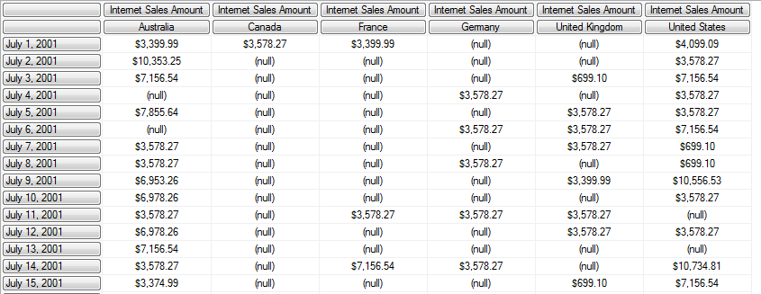
The Customer dimension in Adventure Works isn’t actually very good for illustrating this because customers very rarely buy more than once, but if you look at Countries then you can recreate the scenario. Consider the following query:

select
{[Measures].[Internet Sales Amount]} *
[Customer].[Country].[Country].members on 0,
[Date].[Date].[Date].members
on 1
from [Adventure Works]

image

From the screenshot you can see that on July 1st 2001 there were purchases in 4 out of 6 countries; of those 4 countries, only 2 (Australia and USA) had purchases on July 2nd; both of those had purchases on July 3rd; but by July 4th only USA had seen purchases on every day since the beginning of time.

How then is is possible to get this count of the number of countries that have seen purchases since the beginning of time? I can think of a few approaches. One would involve using recursion and strtoset/settostr, but I generally like to avoid recursion and strtoset because performance can be unpredictable and bad. Probably the best way is to think of the problem like this: if a country has had sales on every day since the beginning of time, then count of days that had sales since the beginning of time will be the same as the total count of days since the beginning of time. Therefore, you can write a query something like this:

with
–count the number of days since the beginning of time
member measures.daycount as
count(null:[Date].[Date].currentmember)

–count the number of non empty days for sales since the beginning of time
member measures.nonemptydaycount as
count(
nonempty(
null:[Date].[Date].currentmember
, [Measures].[Internet Sales Amount])
)

–count the number of countries that have nonemptydaycount = daycount
member measures.[Consistent Customers] as
count(
filter(
[Customer].[Country].[Country].members
, measures.nonemptydaycount = measures.daycount)
)
select measures.[Consistent Customers] on 0,
head([Date].[Date].[Date].members, 15) on 1
from [Adventure Works]

image

Mosha’s technique for optimising count(filter()) calculations might also be useful here, although I have to admit I’ve not tested it to see if it does improve performance.

However, for those of you who are fans of obscure MDX, here’s another solution:

with
member measures.[Consistent Customers] as
count(
–iterate over every date since the beginning of time
generate(
{null : {{[Date].[Date].currentmember} as currentdate}.item(0)}
,
{
–if the current date in the iteration is the first date
iif([Date].[Date].currentmember is [Date].[Date].[Date].members.item(0)
,
–then define the inline named set customerset as
–all the nonempty customers
intersect(
nonempty(
[Customer].[Country].[Country].members
, [Measures].[Internet Sales Amount]) as customerset
, {})
,
–else, redefine the set customerset as the intersection of
–customerset and the nonempty countries in the current time period
intersect(
intersect(
customerset
, nonempty(
[Customer].[Country].[Country].members
, [Measures].[Internet Sales Amount])
) as customerset
, {})
)
–note that the intersect function is used to ensure only an empty
–set is ever returned from these expressions
,
–if the current date in the iteration is the current time period
–ie we are at the final iteration
iif([Date].[Date].currentmember is currentdate.item(0)
–then return the contents of the named set customerset
, customerset
, {})
}
))

select {measures.[Consistent Customers]} on 0,
head(
[Date].[Date].[Date].members
, 15)
on 1
from [Adventure Works]


It uses the generate() function to loop over ever date from the beginning of time to the current time period, and then redefines an inline named set (called customerset) on every step of the iteration to find the non empty countries. It doesn’t perform as well as the previous solution in this particular case, but if there were more countries that might change; a few tweaks to the code might also speed it up. I thought it was worth mentioning, though, for the novelty value.

TopCounts With Ties In MDX

Pretty much everyone that knows MDX knows the TopCount() function, which is used to find the top n items in a set – it can be used for finding your top 10 products, your top 20 salespeople, and so on. However most people don’t consider it’s biggest drawback: it always returns n items, and doesn’t take ties into account.

Consider the following query on Adventure Works, which returns the top 9 dates by Internet Order Count:

SELECT {[Measures].[Internet Order Count]} ON 0,
TOPCOUNT(
[Date].[Date].[Date].MEMBERS
, 9
,[Measures].[Internet Order Count])
ON 1
FROM [Adventure Works]

image

Now look at this query, which does the same thing but returns the top 10 dates:

SELECT {[Measures].[Internet Order Count]} ON 0,
TOPCOUNT(
[Date].[Date].[Date].MEMBERS
, 10
,[Measures].[Internet Order Count])
ON 1
FROM [Adventure Works]

image

Notice how June 11 2004 and June 17 2004 both have the same Internet Order Count of 86, but the latter date isn’t included in the first query. From this you can see that it’s important, when you’re doing a top n query, not to always return n items but to take tied values into account.

Luckily there’s a way of doing this. If you can download and install the dll from the Analysis Services Stored Procedure Project, you can use the TopCountWithTies() function that it provides, like so:

SELECT {[Measures].[Internet Order Count]} ON 0,
ASSP.TOPCOUNTWITHTIES(
[Date].[Date].[Date].MEMBERS
, 9
,[Measures].[Internet Order Count])
ON 1
FROM [Adventure Works]

image

Unfortunately, installing third-party dlls is not always allowed in a production environment, and SSAS 2012 Tabular doesn’t support dlls at all. However there is a way of getting the same result in pure MDX. Here’s an example:

WITH
SET TOP9 AS
TOPCOUNT(
[Date].[Date].[Date].MEMBERS
, 9
,[Measures].[Internet Order Count])
MEMBER MEASURES.TIEDRANK AS
RANK(
[Date].[Date].CURRENTMEMBER
, TOP9
, [Measures].[Internet Order Count])
SET TOP9WITHTIES AS
ORDER(
FILTER(
[Date].[Date].[Date].MEMBERS
, MEASURES.TIEDRANK>0 AND MEASURES.TIEDRANK<=9)
, MEASURES.TIEDRANK
, BASC)

SELECT {[Measures].[Internet Order Count], MEASURES.TIEDRANK} ON 0,
TOP9WITHTIES
ON 1
FROM [Adventure Works]

image

What I’m doing here is first using the TopCount() function to find the set of the top 9 dates (this step isn’t strictly necessary, but it has a significant positive impact on performance), and then using the Rank() function with the third parameter to find the tied rank. The Rank() function should find the position of a member in a set, but when the third parameter for it is specified it doesn’t match members based on the members themselves but on the values of the tuple specified in the third parameter. Hence, even when I have  a date that doesn’t appear in the set TOP9, the Rank() function can still return a value for it if that date has a value for Internet Order Count that does appear in that set.

Validating MDX Queries Without Running Them

Here’s something interesting I came across while looking over some old documentation the other day: a way of checking whether an MDX query is syntactically correct without actually having to run it. You can do this by setting the Content connection string property. The default value for this property is:

Content=SchemaData

And this runs your queries as normal. For example, take the following query on the Adventure Works cube:

select {[Measures].[Internet Sales Amount]} on 0,
[Date].[Calendar Year].members on 1
from [Adventure Works]

On a cold cache I can see lots of activity on Profiler when it’s run, as I’d expect:

image

However, with the connection string set as follows (see here for how to do this in SQL Server Management Studio; but beware – this bug is still around in 2012) :

Content=Schema

When I rerun the query on a cold cache I can see the MDX Script being evaluated but nothing happening for the query:

image

In SQL Server Management Studio the query is executed successfully but no results are returned; notice that in the Resource Usage event all the values are zero too.

If I modify the query to include an error, however:

select {[Measures].[Internet Sales Amount]} on 0,
blah blah blah
[Date].[Calendar Year].members on 1
from [Adventure Works]

I do see an error in SQL Server Management Studio:

image

This functionality could be useful in situations where you wanted to test the syntax of an MDX query or indeed just a calculation – it would allow you to do this without actually running the query and then killing it (and some queries don’t die immediately when they’re cancelled, as you might know).

Technitrain 2013 Course Schedule: SSAS, PowerPivot, MDX, SSIS, TSQL and SQL Server Engine Training in London

As you probably know, when I’m not blogging or wrestling with SSAS I run a small SQL Server training company here in the UK called Technitrain. If you’ve got some training budget to spare and London is convenient for you, you might want to check out the 2013 course schedule below:

As you can see, I’m doing a fair bit of teaching myself but I’m also proud to have Thomas Kejser, Allan Mitchell, Dave Ballantyne, Bob Phillips and Andy Leonard teaching courses for me too. The aim is to deliver reasonably-priced, expert-level Microsoft BI and SQL Server training of the sort the regular training companies don’t provide; it’s basically the kind of training you’d get at a SQLBits or SQL Saturday pre-con but in a more traditional classroom environment and not limited to one day. If you’re reading my blog, you’re my target audience for these courses – so I hope to see you at one of them this year!

Unnecessary All Members and Performance Problems

Maybe an obscure problem, this one, but worth recording nonetheless. The other week I was performance tuning some queries on a customer’s SSAS 2008R2 instance and came across a very strange issue related to the presence of unnecessary All Members in tuples. In this case it was in machine-generated MDX but it’s certainly the case the people new to MDX often include All Members in tuples when they are not actually needed; it’s a not good idea to do this because it can sometimes have unexpected effects as a result of attribute overwrite and because, as I found, it can also cause severe performance problems too.

The problem can be reproduced very easily against Adventure Works on the Customer dimension. Consider the following query that returns a list of customers who bought more than $1000 of goods in 2003:

with
set filteredcustomers as
filter(
[Customer].[Customer Geography].[Customer].members
, ([Measures].[Internet Sales Amount]
, [Date].[Calendar Year].&[2003])>1000)
select
{}
on columns,
filteredcustomers 
on rows
from [Adventure Works]

Pretty straightforward, and it returns instantly on my laptop as I’d expect. However, adding the All Member from the City hierarchy into the tuple used in the filter() function makes the query run very slowly indeed (I killed it after several minutes):

with
set filteredcustomers as
filter(
[Customer].[Customer Geography].[Customer].members
, ([Measures].[Internet Sales Amount]
, [Customer].[City].[All Customers]
, [Date].[Calendar Year].&[2003])>1000)
select
{}
on columns,
filteredcustomers 
on rows
from [Adventure Works]

The All Member here isn’t necessary at all; it won’t affect how the filter works or the set returned at all. Looking in Profiler it seems as though its presence triggers cell-by-cell mode, which is the cause of the awful performance. Interestingly, the performance got worse the more attributes were on the hierarchy – deleting attributes, even when they weren’t used in the query, improved query performance. I’m told the problem could be the result of attribute decoding (which Mosha referred to here, but which I don’t know much else about) as a result of attribute overwrite

Anyway in my case it wasn’t possible to change the MDX because it was being generated by a client tool – the All Member was there because the City hierarchy was being used as a parameter in the query, although in this case nothing had been selected on it. There was a workaround that I found though: it turns out the problem does not occur for user hierarchies that include the key attribute as their lowest level. So, I renamed the City attribute, hid it, and then created a new user hierarchy called City that had Customer as its lowest level:

image

With this done, both of the queries above return instantly.

Introduction to MDX for PowerPivot Users, Part 5: MDX Queries

In part 4 of this series (sorry for the long wait since then!) I finished off looking at what you can do with named sets. Now, before I go on to more important topics like Excel cube functions and calculated members I’d like to take a high-level look at what you can do with MDX queries running against PowerPivot – high level, because there’s much more to MDX queries than can be covered in a single post and, as I explain below, you probably won’t want to do this very often.

So why would I need to write whole queries against a PowerPivot model?

This is a very good question, given that in my opinion 99% of the time you can achieve what you want when building Excel reports using either PivotTables (either with or without named sets) or Excel cube functions. Having said that, the post I wrote a few years ago about binding a table in Excel to an MDX query has been one of the most popular I’ve ever written, so maybe I’m wrong about how frequently people need to do this…

I’d say that you would probably only want to write your own queries when you needed complete control over the MDX and didn’t mind that it made linking the query up to filters or slicers very difficult – for example, if you wanted a list of unpaid invoices, or a list of customers that met some specific criteria, in a dashboard.

Also, when you run MDX queries in Excel you’re going to use an Excel table to show the results rather than a PivotTable. This is actually the format you need to use to pass data to other Excel-based tools like like Excel Data Mining Addins (as well as PowerPivot), so writing your own MDX queries might actually save you having to convert to formulas, as Kasper does here, or cutting/pasting in cases like this.

Why use MDX instead of DAX?

From PowerPivot V2, PowerPivot models can be queried in either MDX or the DAX query language (if you want to learn about DAX queries take a look at the posts I wrote on this topic last year, starting here), and if you’ve already learned a lot of DAX for PowerPivot you’re probably going to be more comfortable using DAX queries. However, I know there are a lot of old SSAS-fans out there doing work with PowerPivot who prefer MDX, and there are still a few things that MDX can do that PowerPivot can’t, so choosing MDX over DAX is a legitimate choice. Examples would be when you want to pivot your resultset and put something other than measures on columns, or show a calculated member on rows, and I show how to do both of these things below.

How do I display the results of an MDX query in Excel?

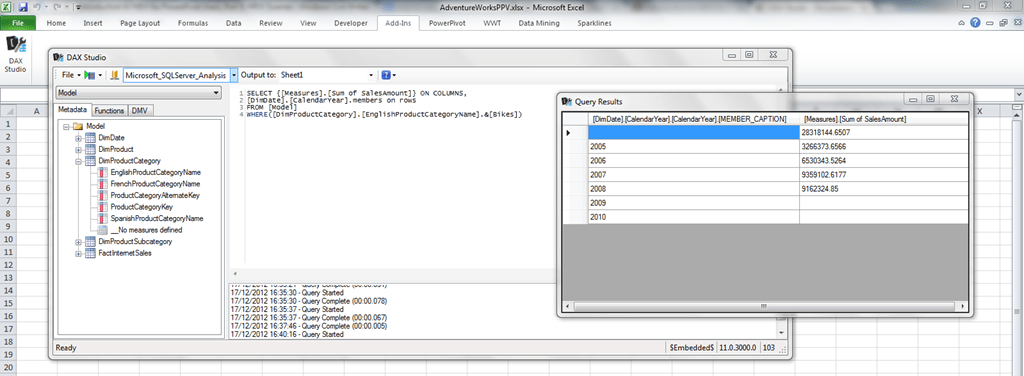
As I said, when you display the results of an MDX query in Excel you’ll need to use an Excel table to do so. I blogged about a few ways to do this here but there’s actually a better way now: using DAX Studio. DAX Studio is a free Excel addin for people who want to write DAX queries against a PowerPivot model, but it can run MDX queries too. Unfortunately it doesn’t display any MDX metadata for you to use – only DAX metadata – but it’s still a much more convenient way of running MDX queries than doing a drillthrough and then editing the query property of a table.

The DAX Studio documentation gives you a good overview of how to use the tool and I won’t repeat that here, but to prove it does work here’s a screenshot of an MDX query run against a PowerPivot model:

image

OK, so get on with it and tell me how to write an MDX query…

The basic MDX query is quite simple. Books online has all the details:

http://msdn.microsoft.com/en-us/library/ms146002.aspx
http://msdn.microsoft.com/en-us/library/ms144785.aspx

…but really all you need to know is this:

Each MDX query needs a SELECT clause. Inside the SELECT clause you need to define one or two axes, either just a columns axis or a columns axis or a rows axis, and the way you define what appears on an axis is using a set, an object we’ve seen a lot of in the last few posts in this series. Each MDX query also needs a FROM clause, with the name of the cube that is to be queried; for PowerPivot the name of the ‘cube’ is always [Model].

Here’s an example of a simple MDX query on a PowerPivot model built on Adventure Works DW that returns a measure on columns and three years on rows:

SELECT
{[Measures].[Sum of SalesAmount]}
ON COLUMNS,
{[DimDate].[CalendarYear].&[2005]
, [DimDate].[CalendarYear].&[2006]
, [DimDate].[CalendarYear].&[2007]}
ON ROWS
FROM [Model]

image

Everything you do on columns, you can do on rows, and vice versa, so:

SELECT 
{[DimDate].[CalendarYear].&[2005]
, [DimDate].[CalendarYear].&[2006]
, [DimDate].[CalendarYear].&[2007]}  
ON COLUMNS,
{[Measures].[Sum of SalesAmount]}
ON ROWS
FROM [Model]

Returns this:

image

Using a set of tuples on rows and/or columns gives a crosstabbed effect:

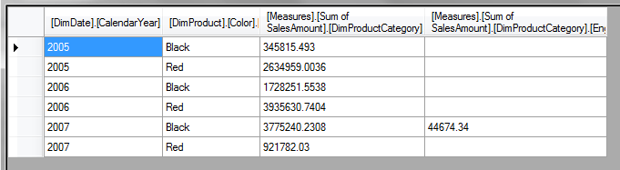
SELECT 
{[Measures].[Sum of SalesAmount]}
*
{[DimProductCategory].[EnglishProductCategoryName].[EnglishProductCategoryName].&[Bikes]
, [DimProductCategory].[EnglishProductCategoryName].[EnglishProductCategoryName].&[Clothing]}
ON COLUMNS,
{[DimDate].[CalendarYear].&[2005]
, [DimDate].[CalendarYear].&[2006]
, [DimDate].[CalendarYear].&[2007]} *
{[DimProduct].[Color].&[Black]
, [DimProduct].[Color].&[Red]}
ON ROWS
FROM [Model]

image

After the FROM clause, you can add a WHERE clause to slice the resultset. Do not confuse the MDX WHERE clause with the SQL WHERE clause: it does something similar but it doesn’t directly affect what appears on rows or columns, it filters the values returned inside the query. For example:

SELECT 
{[Measures].[Sum of SalesAmount]}
ON COLUMNS,
{[DimDate].[CalendarYear].&[2005]
, [DimDate].[CalendarYear].&[2006]
, [DimDate].[CalendarYear].&[2007]}  
ON ROWS
FROM [Model]
WHERE(
[DimProductCategory].[EnglishProductCategoryName].[EnglishProductCategoryName].&[Bikes]
, [DimProduct].[Color].&[Black])

…returns sales for Black Bikes for the years 2005 to 2007:

image

Notice that the Colour Black and the Product Category Bikes don’t appear anywhere on rows or columns, but the values that are shown are for Black Bikes nonetheless.

The WITH clause

You can define your own calculated members (which I’ll talk about in a future post) and named sets inside a query if you add a WITH clause before your SELECT clause. Here’s an example of this:

WITH
SET [MY YEARS] AS
{[DimDate].[CalendarYear].&[2005]
, [DimDate].[CalendarYear].&[2006]
, [DimDate].[CalendarYear].&[2007]}
MEMBER [DimDate].[CalendarYear].[Total 2005-7] AS
AGGREGATE([MY YEARS])
MEMBER [Measures].[Percent of Total] AS
([Measures].[Sum of SalesAmount])
/
([Measures].[Sum of SalesAmount]
, [DimDate].[CalendarYear].[Total 2005-7])
, FORMAT_STRING=’PERCENT’
SELECT 
{[Measures].[Sum of SalesAmount]
,[Measures].[Percent of Total]}
ON COLUMNS,
{[MY YEARS], [DimDate].[CalendarYear].[Total 2005-7]}
ON ROWS
FROM [Model]

image

Here I’ve defined a named set called [MY YEARS] which I’ve then used to define what goes on the rows axis, and two calculated members, [Total 2005-7] which returns the subtotal of the years 2005 to 2007, and a new measure [Percent of Total] that shows the percentage that each row makes up of this subtotal. Incidentally, even though DAX can do this kind of subtotalling, it’s only in MDX that you can define any calculation you want on any axis in your query.

Flattened Rowsets

You might be wondering, looking at the examples above, why the column headers are all in human-unfriendly MDX and why the [Percent of Total] measure hasn’t had any formatting applied. You will also notice in this query how the name of the All Member on the [CalendarYear] hierarchy doesn’t get returned, and you get a blank row name instead:

SELECT 
{[Measures].[Sum of SalesAmount]}
ON COLUMNS,
{[DimDate].[CalendarYear].[All]
,[DimDate].[CalendarYear].&[2005]}
ON ROWS
FROM [Model]

image

This is because, when you run queries that get bound to an Excel table they are returned as flattened rowsets and not cellsets (which is how most SSAS client tools and SQL Server Management Studio returns MDX queries). Basically, this means your nice, multidimensional resultset gets squashed into something tabular – and when this happens, a lot of useful stuff gets lost along the way. Here’s the official documentation on how flattened rowsets are generated:
http://msdn.microsoft.com/en-us/library/windows/desktop/ms716948(v=vs.85).aspx

This is a pain, but there’s no way around it unless you want to write your own code to render a cellset in Excel unfortunately.

Conclusion

Writing your own MDX queries against a PowerPivot model isn’t exactly something you’ll need to do every day, but it’s a useful addition to your PowerPivot toolbox and I wanted to mention it in this series for the sake of completeness. In my next post I’ll be taking a look at MDX calculated members.