Reducing The Number Of Queries Generated By Excel Cube Function Reports On Power BI, Analysis Services And Power Pivot

I am a big fan of using Excel cube functions for reporting on Power BI datasets, Analysis Services and Power Pivot: they allow for a lot more layout flexibility than PivotTables when building reports in Excel. However, they do have a reputation for poor performance and part of the reason for this is their chattiness. While Excel does not generate one query for each cell containing a cube function, it is true that a report using cube functions will generate a lot more MDX queries against your Power BI dataset/Analysis Services cube/Power Pivot mode than the equivalent PivotTable. As a result, one way to improve the performance of reports that use Excel cube functions is to optimise them to reduce the number of MDX queries generated.

To understand how to do this you first need to understand how Excel generates the MDX queries needed by cube functions. First of all it looks at the cells containing CubeValue functions on a worksheet and groups them together by the granularity of the data they are requesting; then, for each granularity, it runs one or more MDX queries to get the data it needs, where each query gets data for up to 500 cells. There’s not much you can do to control this behaviour, but in situations where you have multiple fact tables with different granularities there is a trick you can play to reduce the number of queries.

Let’s take a simple example. Consider the following source data:

…loaded into a Power BI dataset with two fact tables, Sales and Targets, and two dimension tables, Product and Country:

Now consider the following report that uses two groups of cube formulas to get the Sales Amount for Apples in the UK and the Target Amount for the UK:

Here are the formulas for these cells:

This worksheet generates two MDX queries for the two different granularities (plus one other MDX query that gets some metadata). The first gets the Sales Amount for Apples in the UK and populates the CubeValue function in cell D3. This query consists of a single MDX tuple whose granularity is Country, Measure and Product:

SELECT 
{([Country].[Country].&[UK],[Measures].[Sales Amount],[Product].[Product].&[Apples])} 
ON 0 
FROM [Model] 
CELL PROPERTIES VALUE, FORMAT_STRING, LANGUAGE, BACK_COLOR, FORE_COLOR, FONT_FLAGS

The second gets the Target Amount for the UK and populates the CubeValue function in cell D6. It consists of a single MDX tuple whose granularity is Country and Measure:

SELECT 
{([Country].[Country].&[UK],[Measures].[Target Amount])} 
ON 0 
FROM [Model] 
CELL PROPERTIES VALUE, FORMAT_STRING, LANGUAGE, BACK_COLOR, FORE_COLOR, FONT_FLAGS

It is possible to get the same data in a single MDX query and the key to doing so is to make the granularity of the two requests the same. One way of doing this is to edit the contents of cell D6, which at this point contains the following formula to get the Target Amount (in D5) for the UK (in C6) using the CubeValue function:

=CUBEVALUE("CubeFunctionsOptimisationDataset", C6,D5)

If you add an extra reference to cell C3, which contains the CubeMember function returning the Product Apples, like so:

=CUBEVALUE("CubeFunctionsOptimisationDataset", C6,D5, C3)

Then this results in exactly the same data being returned to Excel and exactly the same data being displayed in the worksheet, but with a single MDX query being generated:

SELECT 
{([Country].[Country].&[UK],[Measures].[Target Amount],[Product].[Product].&[Apples]),
([Country].[Country].&[UK],[Measures].[Sales Amount],[Product].[Product].&[Apples])} 
ON 0 
FROM [Model] 
CELL PROPERTIES VALUE, FORMAT_STRING, LANGUAGE, BACK_COLOR, FORE_COLOR, FONT_FLAGS

As you can see, this query now consists of two tuples whose granularity is Country, Measure and Product. The reason this works is because adding the reference to the Product Apples makes no difference to the value returned by the Target Amount measure – which has no relationship with the Product dimension table – but it is enough to fool Excel into thinking that the CubeValue function in cell D6 is making a request at the same granularity as the CubeValue function in cell D3. It is necessary to add a reference to an individual Product, such as Apples, rather than the All Member on Product though.

Another, perhaps more complicated, way of achieving the same result is to leave the formula in cell D6 the same but change the formula in C6 from:

=CUBEMEMBER("CubeFunctionsOptimisationDataset", "[Country].[Country].[All].[UK]")

…to use the tuple form of CubeMember to get the combination of Apples and UK:

=CUBEMEMBER("CubeFunctionsOptimisationDataset", {"[Product].[Product].[All].[Apples]","[Country].[Country].[All].[UK]"})

Note that when you use this tuple form of CubeMember, putting Apples first in the tuple and Country second results in only the Country name being displayed in the cell, so again the data displayed in Excel is exactly the same.

Reducing the number of MDX queries in this way can improve performance for two reasons: it reduces the number of round trips to the dataset and it gives the Analysis Services engine (in Power BI, Analysis Services or Power Pivot) the chance to get the data needed in a more optimal way than might be possible with multiple queries. I don’t think the technique in this post will make a massive difference to performance but if you do try this, I’m curious to see how much of an improvement you see.

Sharing Excel Reports Connected To Power BI Datasets Or The Excel Data Model/Power Pivot Using OneDrive For Business

I love Excel as an alternative to Power BI reports, especially now that Excel Online allows you to interact with browser-based Excel reports that use Power BI datasets or the Excel Data Model (aka Power Pivot) as a source. After all, why try to recreate a PivotTable in a Power BI report when you can give your users an actual PivotTable? You can publish Excel reports to Power BI and view them there; however if you want to share these reports using OneDrive for Business, outside Power BI, you’ll need to think carefully about how you do so before you allow other people to view the report.

To illustrate the problem I used Power Pivot to load some data into the Excel Data Model, built a simple report with a PivotTable and PivotChart, saved it to OneDrive for Business and then opened it in the browser with Excel Online. As you can see it’s possible to interact with the report in the browser, changing slicers and moving fields around in the PivotTable and PivotChart field lists:

So far so good. However, an Excel file saved to OneDrive for Business is a shared document – and any changes that one user makes are immediately visible to all other users who have access with full Edit permissions. This means that if you change a slicer and someone else is viewing my report at the same time, they will see the slicer change too in real-time. This may be useful in scenarios where you are collaborating with someone on the same report and want them to see your changes, but in most cases this is not desirable behaviour for a report. Here’s an example with the same Excel report open side by side in Chrome and Edge:

How can you stop this happening? One option is to use View mode. When an Excel workbook is in View mode a user can interact with slicers and move fields around in the PivotTable without these changes affecting other users and without these changes being saved; they cannot make most other changes such as entering values in cells. If users do have full Edit permissions they can always switch to View mode using the dropdown menu in the top right corner of the screen:

You can also use the Protect Workbook option to make sure users open the workbook in View mode by default. However there is always the danger that if a user has Edit permissions they will switch to Edit mode and make unwanted changes, so as a result it’s better to share the workbook without Edit permissions using the “Can View” option described here so they can only open the workbook in View mode:

There is another option: using an Embed link. To get this, click on the File menu in Excel Online and then on the backstage view select Share and then Embed:

As the UI suggests, this option is intended for scenarios where you want to embed your workbook in another application; it’s similar to View mode but a bit more restrictive. In the Embed dialog that opens you can choose which parts of the workbook to share, whether grid lines are shown and other useful options:

Here you need to select the “Let people sort and filter” option otherwise your users won’t be able to use the slicers. Next, copy the code from the “Embed code” box and paste into your favourite text editor so you can extract the URL in the src tag – this is the URL you should give to your users. When a user opens an Excel report using a link generated in this way they won’t see the Excel ribbon at all; they can interact with slicers but can’t get access to the PivotTable fields pane and so won’t be able to move fields around, for example changing what is on rows or columns. I think this gives the best experience for end users who just want to view an Excel report in the browser.

Note that this does not replace normal OneDrive for Business sharing and permissions though: you’ll still need to share the report with your users, ideally with “Can View” permissions as described above. If your Excel report connects back to a Power BI dataset you also need to ensure that your users have the appropriate permissions on that dataset, which means they’ll either need to be at least a Member in the workspace the dataset is stored in or have Build permissions.

What-If Analysis With Excel Power Pivot: Automatically Refreshing Individual Tables In The Excel Data Model Using VBA

Sometimes, when you’re analysing data, you need to be able to change variables and see what the impact is: for example you might want to see what your profit margin looks like if tax rates are set at different levels. Power BI’s what-if parameter feature can do this but it has the limitation that you can’t enter any value you like – you need to create a table containing all possible variable values in advance. The advantage the Excel Data Model/Power Pivot has over Power BI for this type of what-if analysis is that you have the Excel worksheet available, which is not only a place to display your report but which can also be used as a data source for tables in the Excel Data Model, making it easy for users to enter whatever variable they want. Up until recently, though, I assumed that if you were importing data from the worksheet into the Excel Data Model you would need to take some form of manual action, for example clicking a refresh button, to load the new data from the worksheet into the Excel Data Model when the data there changed. In this blog post I’ll show you how you can use VBA to solve this problem and build an elegant what-if analysis solution in Excel where no extra clicks are needed.

Let’s look at a very simple example. Here’s a very simple model in Excel with two tables, Sales (containing sales data) and TaxRate (which has just one row and column, a number representing a tax rate):

Here are the measure definitions:

Sales Amount:=SUM(Sales[Sales])
Entered Tax Rate:=MAX('TaxRate'[Tax Rate])
Tax Paid:=[Sales Amount]*[Entered Tax Rate]

The source for the Sales table doesn’t matter, but let’s assume that it’s so large that we don’t want to wait to reload the data if we don’t have to. The source for the TaxRate table is a named range on the worksheet, also called TaxRate:

The data from this named range is loaded into the Excel Data Model using a Power Query also called TaxRate:

let
    Source = Excel.CurrentWorkbook(),
    TaxRate = Source{[Name="TaxRate"]}[Content],
    #"Changed Type" = Table.TransformColumnTypes(TaxRate,{{"Column1", type number}}),
    #"Renamed Columns" = Table.RenameColumns(#"Changed Type",{{"Column1", "Tax Rate"}})
in
    #"Renamed Columns"

Here’s the fun bit. What we want to do is automatically refresh just the TaxRate table in the Excel Data Model when someone changes the value in the TaxRate named range on the worksheet, and you can do that with the following VBA (shamelessly adapted from this example in the docs) on the worksheet with the named range on:

Private Sub Worksheet_Change(ByVal Target As Range)
    Dim KeyCells As Range

' The variable KeyCells contains the cells that will
    ' cause an alert when they are changed.
    Set KeyCells = Range("TaxRate")

If Not Application.Intersect(KeyCells, Range(Target.Address)) _
           Is Nothing Then

'Refresh the TaxRate Power Query query
        ActiveWorkbook.Queries("TaxRate").Refresh

End If
End Sub

As I mentioned in this post from earlier this year, you can now refresh individual Power Query queries in VBA; what I’ve just realised is that this means you can refresh individual tables in the Excel Data Model from VBA, without having to refresh all the tables (which could be very slow). Actually, it looks like it has been possible to refresh individual tables in the Excel Data Model for a long time using the ModelTable.Refresh method but I guess I didn’t think about this problem until I knew about the Power Query refresh change.

Here’s the end result:

As you can see, as soon as the tax rate is changed in the worksheet it’s loaded automatically into the Excel Data Model and the new value is used in the measures shown in the PivotTable almost immediately. This makes what-if analysis much easier and I can think of several scenarios where this kind of automatic refresh would be useful too, but I’ll leave them for a future blog post.

Filtering An Excel Cube Function Report By A List Of Manually-Entered Values

In Power BI there’s a popular custom visual called “Filter by list” that lets you filter a Power BI report by any list of values that you paste into it. It can save you a lot of time in some scenarios, for example if you need to copy a list of values from another application and select those values in a slicer. In this post I’ll show how to recreate the same functionality in an Excel report connected to Power BI, Analysis Services or the Excel Data Model/Power Pivot using cube functions and dynamic arrays.

To show how I’m going to use a super-simple model built using Power Pivot consisting of the following single table:

The only other thing to note about the model is that it contains a measure called Sales Amount that sums up the values in the Sales column:

Sales Amount:=SUM(Sales[Sales])

Here’s what a PivotTable connected to this model looks like:

The aim here is to recreate this PivotTable using cube functions and allow the user to enter the list of invoice numbers used to slice the data either manually or by copy-and-pasting them into a table.

The first step is to create an Excel table (which I’ve called InvoiceNumbers) to hold the invoice numbers the user enters:

The next thing to do is to generate the text of the MDX set expression representing the list of invoice numbers in this table, which I’ve put in cell D2:

="{" & TEXTJOIN(",",TRUE, "[Sales].[Invoice Number].[Invoice Number].&[" & InvoiceNumbers & "]" ) &"}"

This text is used to create two named sets using the CUBESET function. The first, which I’ve put in cell D3, simply returns the set of invoice numbers that you get from evaluating the above MDX expression:

=CUBESET("ThisWorkbookDataModel", $D$2, "Invoice Numbers")

The second named set, in D4, is more complicated: it returns the set of customers that have sales for these invoice numbers.

=CUBESET(
"ThisWorkbookDataModel", 
"NONEMPTY( [Sales].[Customer].[Customer].MEMBERS, {[Measures].[Sales Amount]} * " & $D$2 & ")",
"Customers")

Last of all are the cube functions that display the report itself. In cell E6 is the CUBEVALUE function returning the measure Sales Amount:

=CUBEMEMBER("ThisWorkbookDataModel", "[Measures].[Sales Amount]")

In D7 is the formula (using the technique I blogged about here) to get the list of Customers returned by the second named set above:

=MAKEARRAY(
CUBESETCOUNT($D$4), 
1, 
LAMBDA(r,c, CUBERANKEDMEMBER("ThisWorkbookDataModel", $D$4, r))
)

Finally, in D8, is the expression that gets the Sales Amount values for each customer, sliced also by the set of selected invoice numbers:

=MAKEARRAY(
CUBESETCOUNT($D$4),
1,
LAMBDA(r,c,
CUBEVALUE("ThisWorkbookDataModel", INDEX($D$7#,r), $D$3, $E$6))
)

Here are the formulas all together:

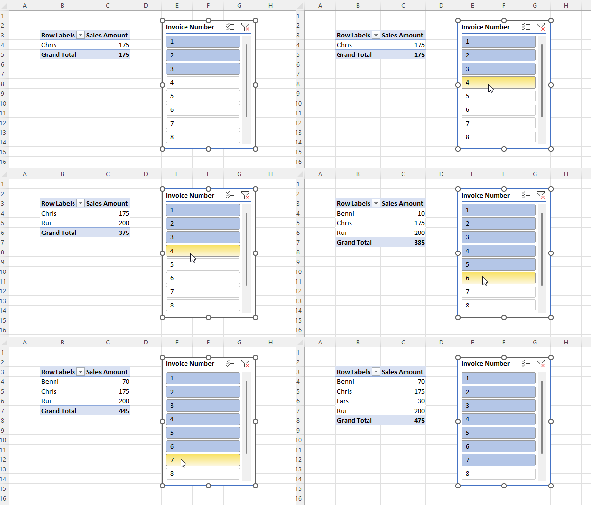
And here it all is working:

One last point: to keep things simple I’ve not included any error handling, which means that if a user enters a blank value or a value that isn’t an invoice number in the table the whole thing will break. To handle errors using the technique I blogged about here, alter the formula in D2 to:

="{"&
TEXTJOIN(
",",
TRUE,
LET(
MemberExpression,
"[Sales].[Invoice Number].[Invoice Number].&["&InvoiceNumbers&"]",
"IIF(ISERROR(STRTOMEMBER("""&MemberExpression&""")), {}, STRTOMEMBER("""&MemberExpression&"""))")
) &"}"

You can download the example workbook here (although it may not work unless you’ve got a version of Excel with dynamic arrays enabled).

Refreshing Power Pivot Excel Data Models That Use The Current Workbook As A Data Source In Excel Online

Something that got lost in all the excitement around Excel reports connected to Power BI datasets working in Excel Online is the fact that Excel reports connected to the Excel Data Model – aka Power Pivot – now work too (although I did mention it here). Right now it’s not possible to refresh the data stored in the Excel Data Model if you are connected to external data sources. However, today I noticed something nice: if you are using a, Excel table in the same workbook as a source for a table in the Excel Data Model, if you make a change to the table in the worksheet then it is possible to refresh the data in the Excel Data Model.

Here’s an example. In Excel on the Desktop I created a new workbook and added a simple table to a worksheet:

I then moved to the Power Pivot tab on the ribbon and clicked the “Add to Data Model” button to add this table to the Excel Data Model:

I then created a PivotTable connected to the Excel Data Model:

After saving the workbook to OneDrive for Business, I closed it in Excel Desktop and reopened it in Excel Online in the browser:

Finally I was able to change a value in the source table, click the Refresh Selected Connection button on the Data tab in the ribbon, and see the change reflected in the PivotTable connected to the Excel Data Model:

Of course it would be better if you could refresh external data sources too but I still think this could be useful, for example if you had multiple users updating forecasts or budgets in an Excel table in the browser and were using the Excel Data Model for reporting on this data.

Excel Cube Functions, Dynamic Arrays And Lambdas, Part 3: Grouping And Histograms

In the last post in this series I showed how you can use Excel’s new Lambda helper functions to return tables. In this post I’ll show you how you can use them to return a dynamic array of CubeSet functions which can be used to build a histogram and do the kind of ABC-type analysis that can be difficult to do in a regular Power BI report.

For the examples in this post I added some rows to the Excel Data Model table that I’m using to hold my source data:

The aim here is to put these products into an arbitrary number of groups, or buckets, based on their sales. To define these buckets I created another Excel table called Buckets that has three columns: the name of the bucket, and the lower bound and the upper bound of the sales amount that determines whether a product should fall into the bucket:

I then created two dyanmic array formulas using the new Map function. In cell G2 I added this formula:

=
MAP(
 Buckets[Bucket Name], 
 Buckets[Lower Bound], 
 Buckets[Upper Bound], 
 LAMBDA(
  n,
  l,
  u, 
  CUBESET(
   "ThisWorkbookDataModel", 
   "FILTER([Sales].[Product].[Product].MEMBERS, [Measures].[Sales Amount]>=" & l & 
   " AND [Measures].[Sales Amount]<=" & u & ")", 
   n)
  )
)

And in cell H2 I added this formula:

MAP(
 G2#, 
 LAMBDA(
  s, 
  IF(
   CUBESETCOUNT(s)>0, 
   CUBEVALUE(
    "ThisWorkbookDataModel", 
    s, 
    "[Measures].[Sales Amount]"),
   0)
  )
)

Here’s what these two formulas return:

The formula in G2 takes three arrays – the values from the three columns in the Buckets table – and then loops over the values in those columns and uses the CubeSet function to return a set of the Products whose sales are between the lower and upper bounds. Since there are two rows in the Buckets table, this formula returns two sets. The formula in H2 uses the CubeValue function to return the aggregated sales amount for each set.

Last of all I created a column chart bound to the values in G2 and H2. This was a bit tricky to do, but I found the answer in this video from Leila Gharani – you need to create names that return the contents of the ranges G2# and H2# and then use the names in the chart definitions.

The beauty of all this is what when you edit the ranges in the Buckets table in the top left of the worksheet, edit the names of the buckets or add new buckets, the table and chart update automatically.

After doing all this I realised there was another, probably easier way to achieve the same result without using the Map function. All I needed to do was to add new calculated columns to the bucket table to return the sets and values:

Here’s the formula for the Set column in the table above:

=CUBESET(
"ThisWorkbookDataModel", 
"FILTER([Sales].[Product].[Product].MEMBERS, [Measures].[Sales Amount]>=" & 
[@[Lower Bound]] & 
"AND  [Measures].[Sales Amount]<=" & 
[@[Upper Bound]] & 
")", 
[@[Bucket Name]] & 
" set"
)

…and here’s the formula for the Sales column in that table:

= IF(
CUBESETCOUNT(
[@Set])>0, 
CUBEVALUE(
"ThisWorkbookDataModel", 
[@Set], 
"[Measures].[Sales Amount]"
),
0
)

I think this second approach should work with any version of Excel since the introduction of tables and cube formulas.

Excel Cube Functions, Dynamic Arrays And Lambdas, Part 2: Returning Tables

In the first post in this series I showed how to use the new Excel Lambda helper functions to return an array containing all the items in a set. That isn’t very useful on its own, so in this post I’ll show you how to generate an entire dynamic table using Excel cube functions and Lambda helper functions.

In this post I’ll be using the same source data as in my previous post: a table containing sales data with just two columns.

With this table added to the Excel Data Model/Power Pivot, I created two measures:

I then created created two sets using CubeSet containing the sets of Products (in cell B2 of my worksheet) and Measures (in cell B4) to use in my table:

=CUBESET("ThisWorkbookDataModel", "[Sales].[Product].[Product].MEMBERS", "Product Set")

=CUBESET("ThisWorkbookDataModel", "{[Measures].[Sales Amount], [Measures].[Forecast Sales]}", "Measure Set")

Here are the formulas shown in the worksheet:

And here’s the output – remember you only see the text in the third parameter displayed in the cell:

Now, here’s the fun part – a single formula that takes these sets and builds a table with the Measures on columns and the Products on rows:

=MAKEARRAY(
  CUBESETCOUNT(B2)+1,
  CUBESETCOUNT(B4)+1,
  LAMBDA(r,c,
   SWITCH(
    TRUE(),
    AND(r=1,c=1),
    "",
    c=1,
    CUBERANKEDMEMBER("ThisWorkbookDataModel",$B$2,r-1),
    r=1,
    CUBERANKEDMEMBER("ThisWorkbookDataModel",$B$4,c-1),
    CUBEVALUE("ThisWorkbookDataModel",
     CUBERANKEDMEMBER("ThisWorkbookDataModel",$B$2,r-1),
     CUBERANKEDMEMBER("ThisWorkbookDataModel",$B$4,c-1)
    )
   )
  )
)

Here’s what this formula returns:

How does this work? Going through the MakeArray function step-by-step:

  • The first two parameters specify that the output will be an array with one more row than there are items in the Product set and one more column than there are items in the Measures set.
  • The third parameter returns a Lambda that is called for every cell in this array. This Lambda contains a Switch with the following conditions:
    • For the top-left cell in the array, return a blank value
    • In the first column, use the CubeRankedMember function to return the Products on the rows of the table
    • In the first row, use the CubeRankedMember function to return the Measures on the columns of the table
    • In the body of the table, use the CubeValue function to return the values

Here’s a slightly more ambitious version that returns the same table but adds a total row to the bottom:

=
LET(
 NumberOfRows,
 CUBESETCOUNT(B2)+2,
 NumberOfColumns,
 CUBESETCOUNT(B4)+1,
 MAKEARRAY(
  NumberOfRows,
  NumberOfColumns,
  LAMBDA(r,c,
   SWITCH(
    TRUE(),
    AND(r=1,c=1),
    "",
    AND(r=NumberOfRows,c=1),
    "Total",
    r=NumberOfRows,
    CUBEVALUE("ThisWorkbookDataModel",
     $B$2,
     CUBERANKEDMEMBER("ThisWorkbookDataModel",$B$4,c-1)),
    c=1,
    CUBERANKEDMEMBER("ThisWorkbookDataModel",$B$2,r-1),
    r=1,
    CUBERANKEDMEMBER("ThisWorkbookDataModel",$B$4,c-1),
    CUBEVALUE("ThisWorkbookDataModel",
     CUBERANKEDMEMBER("ThisWorkbookDataModel",$B$2,r-1),
     CUBERANKEDMEMBER("ThisWorkbookDataModel",$B$4,c-1))
    )
   )
  )
)

Two extra things to note here:

  • This is a great example of a complex formula where the new Excel Let function can be used to improve readability and prevent the same value being evaluated twice.
  • The values in the Total row are calculated in the Excel Data Model, not on the worksheet, by using the CubeSet function inside the CubeValue function. This means that the totals will be consistent with what you see in a PivotTable and therefore correct

This is still very much a proof-of-concept. I need to look at the performance of this approach (it may not be optimal and may need tuning), and I’m not sure how a table like this could be formatted dynamically (especially the Total row). It is exciting though!

Excel Dynamic Arrays And The CubeSet Function

Among all the exciting announcements made at Ignite last week, one you may have missed (even in all the Excel-related announcements here) was that dynamic arrays have finally reached GA. Ever since they were announced I’ve been interested in how they can be used with Excel cube functions, which allow you to get data from Analysis Services, Power BI and the Excel Data Model/Power Pivot into cells on the worksheet, and I’ve blogged about this once already. Even though right now the CubeValue function can’t be used with dynamic arrays – alas – there are still some interesting ways dynamic arrays and cube functions can be used together and in this post I’ll show you another one I’ve found.

Say you have the following set of tables in the Excel Data Model:

image

And the following measure that counts the number of customers who bought something:

[sourcecode language='html'  padlinenumbers='true']
Distinct Customers:=DISTINCTCOUNT('Internet Sales'[CustomerKey])
[/sourcecode]

Let’s also say you have on a worksheet the following table of data showing the number of distinct customers broken down by product, created using the CubeMember and CubeValue functions:

image

Here are the formulas for this table:

image

So far, all very straightforward. Now let’s say you want to use a dynamic array to filter the rows in this table so you only see the products that have more than a certain number of distinct customers, and you want to see a grand total for this filtered list of customers, like so:

ExcelDynamicArray

Here are the formulas to achieve this:

image

To explain what’s going on here:

  • Cell C2 contains the text “ThisWorkbookDataModel”, the name of the connection to the Excel Data Model. Doing this makes the other Excel formulas here much easier to read!
  • Cell F2 – which I’ve turned into a named range called FilterThreshold – contains the number of customers which a product must exceed to be shown.
  • Cell E5 contains the dynamic array Filter function that filters the rows shown in the first two screenshots above and only returns the products that exceed the threshold. The formula is:
    FILTER(B5:B134,C5:C134>FilterThreshold)
  • Cell E6 does something similar to E5 but returns the number of distinct customers for each product. If all I wanted was the products and the number of distinct customers I wouldn’t have needed two separate formulas, I could have used one, but I need to add the grand total too…
  • Cell E4 contains the formula:
    CUBESET($C$2, E5#, “Total”)
    This creates a set from the spill reference E5#, which contains the cells containing CubeMember formulas returned by the Filter function. For some reason CubeSet returns an error if you try to use a dynamic array formula in its second parameter but using a spill reference works ok; this is why I had to use separate formulas in E5 and E6.
  • Finally, cell F4 contains the formula that returns the total distinct count for all products returned in the filtered list using CubeValue and the set created in cell E4:
    CUBEVALUE($C$2, “[Measures].[Distinct Customers]”, E4)
    Since this is a distinct count the only way to get the correct value here is using CubeSet, CubeValue and the DAX measure – there would be no way to calculate the correct value using Excel formulas. The same could be said of almost any other DAX measure that wasn’t a simple aggregation.

You can download the sample workbook for this post here.

Obscure MDX Month: Deselecting Members In An Excel PivotTable Leads To Missing Rows

Here’s some interesting (and borderline buggy) Excel PivotTable behaviour I learned about today from Charles-Henri Sauget, as well as the workaround for it courtesy of the great Greg Galloway.

Say you have a large dimension attribute hierarchy with 200,000 members on it in SSAS MD (or the equivalent in Tabular or Power Pivot) and drop it onto the rows of an Excel PivotTable. As you would expect, you get a PivotTable with 200,000 rows in it:

image

However if you then deselect just one member on rows like so:

image

…you’ll find that the PivotTable does not have 199,999 rows – in Excel 2016 it only has 32,000 rows:

image

(different versions of Excel may return different numbers of rows here, but still not the full number).

If you look at the MDX generated by Excel it consists of all of the member unique names that are still selected, and unsurprisingly it’s a gigantic query:

image

However, it turns out you can make Excel do the sensible thing and use the Except() function to return everything apart from the deselected member by going to the Field Settings dialog and selecting “Include new items in manual filter”:

image

image

This then gives you the expected number of rows in the PivotTable:

image

I suspect the reason Excel is generating the crazy-long MDX statement by default is that it’s the only way to prevent new members being added to the PivotTable if they are added to the attribute hierarchy in future. On a really large attribute hierarchy, though, the risk is that the resulting MDX query might exceed the maximum length of a query, so Excel has to truncate the number of members returned to make the query shorter. With “Include new items in manual filter” selected, though, it’s ok if new members do get added to the PivotTable in the future so it’s ok to use the Except() function in the query.

Handling Missing Members In The CubeSet() Function With Power Pivot

Last week I received an email from a reader asking how to handle missing members in MDX used in the Excel CubeSet() function. My first thought was that this could be solved easily with the MDXMissingMemberMode connection string property but it turns out this can’t be used with Power Pivot in Excel 2013/6 because you can’t edit the connection string back to the Excel Data Model:

image

Instead, you have no choice but to handle this in MDX.

Here’s an illustration of the problem. Imagine you have the following table of data on your Excel worksheet:

image

With this table added to the Excel Data Model, you could write the following Excel formula using CubeSet():

[sourcecode language=”text” padlinenumbers=”true”]
=CUBESET(
"ThisWorkbookDataModel",
"{[Sales].[Product].[All].[Apples],
[Sales].[Product].[All].[Oranges],
[Sales].[Product].[All].[Pears]}",
"Set")
[/sourcecode]

image

In the screenshot above the CubeSet() formula is used in H3, while in H4 there’s a formula using CubeSetCount() that shows the set contains three members.

If the source data is updated so that the row for Pears is deleted like so:

image

Then the CubeSet() formula returns an error because the member Pears no longer exists:

image

How can this be avoided? If what you actually wanted was all of the Products, whatever they were, the best thing to do is to use the MDX Members function like so:

[sourcecode language=”text”]
=CUBESET(
"ThisWorkbookDataModel",
"{[Sales].[Product].[Product].MEMBERS}",
"Set")
[/sourcecode]

[I talk about the Members function in this post in my series of posts on MDX for Power Pivot users]

This formula does not return an error and you can see that the CubeSetCount() formula below shows the set only contains two members now:

image

If you do need to refer to individual members then the MDX you need is more complicated:

[sourcecode language=”text”]
=CUBESET(
"ThisWorkbookDataModel",
"{[Sales].[Product].[All].[Apples],
[Sales].[Product].[All].[Oranges],
iif(
iserror(
strtomember(""[Sales].[Product].[All].[Pears]"")
),
{},
{strtomember(""[Sales].[Product].[All].[Pears]"")}
)
}",
"Set")
[/sourcecode]

image

This MDX uses the StrToMember() function to interpret the contents of a string as an MDX expression returning a member; if this expression returns an error then it is trapped by the IsError() function and an empty set is returned.

This isn’t particularly pretty, though, and ideally the MDXMissingMemberMode connection string property would be set to Ignore in the Excel Data Model connection string property.