SSAS 2016 Locking Improvements

I first became aware of the server-wide lock taken out by SSAS when processing finishes – and the issues that this can cause – from this blog post by Andrew Calvett back in 2009. More information on how locking works in SSAS can be found in chapter 26 of “Microsoft SQL Server 2008 Analysis Services Unleashed”, while the most comprehensive discussion of this topic can be found in this post by Jason Howell:
https://blogs.msdn.microsoft.com/jason_howell/2012/07/03/analysis-services-stops-accepting-new-connections-processing-commit-locks-hurt/

Over the years I’ve worked with several customers who have run into locking problems as a result of users querying while processing or synchronisation are taking place, so as a result I was interested to read the following paragraph in the white paper on “Automated Partition Management For Analysis Services Tabular Models” that was published a few months ago:

Note that commit operations have been optimized considerably for tabular models in SQL Server 2016. This has caused noticeable improvements in locking and blocking for some customers with near-real time processing requirements. Database write-commit locks are required to safely complete tasks such as merging pending changes, persisting files to disk, clearing some cached state, deletion of old files, etc. In previous versions of Analysis Services, a server-level write commit lock was taken while most of these tasks were performed. With SQL Server 2016, the server-level locks are far more limited; they are only taken while producing the delta of transaction updates, and are then immediately released.

This is very good news, and in fact the improvements apply to SSAS Multidimensional 2016 as well as SSAS Tabular 2016. The ever-helpful Akshai Mirchandani of the dev team has given me more details on the changes, so here’s a summary of what happens during a commit operation and what’s new in SSAS 2016:

  • First of all, a database read-commit lock is taken to analyse all the pending changes.
  • Next a database write-commit lock is taken so that the transaction can be committed safely. This is the lock that can be blocked by long-running queries, and this is where the ForceCommitTimeout property comes into play with the result that these long-running queries may get cancelled.
  • This lock is held while the pending changes are merged together.
  • At this point SSAS is ready to do the commit, and where it takes a server-level write-commit lock. This is also the point where the improvements in SSAS 2016 have been made.
    • In previous versions SSAS would update the master.vmp file in place and hold the server-level write-commit lock while that happens and while some other, potentially time-consuming things like clearing cached state and deleting all the old files take place. This could in some cases result in the server-level write-commit lock being held for an extended period.
    • Instead in SSAS 2016 a delta of all the transaction updates are written to a .txn file, and after that the server commit lock is released. The time-consuming tasks mentioned in the previous bullet still take place but after the server-level write-commit lock has been released. This means the server-level write-commit lock is now held for a very short amount of time, and what’s more that amount of time is quite consistent.
  • Finally, all remaining locks such as the database write-commit lock are released.

I haven’t had a chance to test these changes in a production system yet but it sounds like anyone that needs to process or synchronise regularly throughout the day will benefit from upgrading to SSAS 2016.


Finding Out (Approximately) How Long A Calculation Contributes To The Duration Of An MDX Query

In my last two blog posts (see here and here) I showed how to use the Calculation Evaluation and Calculation Evaluation Detailed Information trace events to work out which MDX calculations are evaluated when a query runs in Analysis Services Multidimensional. That’s very useful, but wouldn’t it be great if you could work out how long any single calculation contributes to the overall duration of a query? If you could, it would make performance tuning MDX calculations much easier.

While you can’t get an exact amount of time taken for each calculation, the good news is that it is possible to get a duration rounded to the next second if your calculation is evaluated in bulk mode.

Take a look at the following query:

[sourcecode language='text'  padlinenumbers='true']
WITH

MEMBER MEASURES.DAYRANK AS
RANK(
[Date].[Date].CURRENTMEMBER, 
[Date].[Date].[Date].MEMBERS)-1

MEMBER MEASURES.HADSALE AS
IIF(
[Measures].[Internet Sales Amount]=0,
NULL,
MEASURES.DAYRANK)

MEMBER MEASURES.LASTSALERANK AS
MAX(
NULL:[Date].[Date].CURRENTMEMBER, 
MEASURES.HADSALE)

MEMBER MEASURES.LASTSALE AS
([Measures].[Internet Sales Amount], 
[Date].[Date].[Date].MEMBERS.ITEM(MEASURES.LASTSALERANK))

MEMBER MEASURES.SIMPLECALC AS
[Measures].[Internet Sales Amount] * 2

SELECT 
HEAD([Customer].[Customer].[Customer].MEMBERS, 200)
*
{MEASURES.SIMPLECALC, MEASURES.LASTSALE}
ON 0,
[Date].[Date].[Date].MEMBERS
ON 1
FROM
[Adventure Works]
[/sourcecode]

This query contains five calculated measures: the first four in the WITH clause, DAYRANK, HADSALE, LASTSALERANK and LASTSALE, are based on my approach for finding the last ever non-empty value for a measure across time; the final measure, SIMPLECALC, is as the name suggests a very simple calculation. On my laptop this query takes around 13 seconds to run on my laptop, on a warm Storage Engine cache. Why does it take so long? It’s clearly the calculations that are the problem, but which one(s)?

Luckily all of the calculations in this query are evaluated in bulk mode so, as I discussed in my last two posts, there is an event raised with:

Event Class = Calculation Evaluation Detailed Information

Event Subclass = 107 – RunEvalNode Finished Calculating Item

…for each of the calculations when they are evaluated. Unfortunately the Duration column for this event always shows 0, but there is a way to see approximately how long the calculation took by comparing the Start Time and Current Time columns in the trace.

The 107 – RunEvalNode event for the measure SIMPLECALC shows the same time for the Start Time and Current Time columns:

image

This indicates that the SIMPLECALC calculation is evaluated in under a second.

However, sequence of 107 – RunEvalNode events for the LASTSALE calculation shows something different:

image

There’s a gap of 7 seconds between the StartTime and the CurrentTime, and this indicates that the calculation took 7 seconds to evaluate. It’s a bit frustrating that there isn’t a way to get a more accurate duration here, but it’s still very clear which calculation is taking all the time. Even though the time for calculating LASTSALE includes the time taken for calculating LASTSALERANK, HADSALE and DAYRANK (all of which need to be calculated in order to calculation LASTSALE), the equivalent rows in the trace for these other calculations show they took under a second each. It’s only the logic inside LASTSALE itself that is slow – so that’s where any tuning needs to take place. Indeed, modifying the query to return LASTSALERANK instead of LASTSALE makes the query faster by around 6 seconds, supporting this conclusion.

If you’re curious about what the other 6 seconds of the query execution time is taken up by, it seems like it’s serialisation of the results – something I blogged about here. The query returns a cellset with 400*1190=476000 cells in, and SSAS doesn’t cope well with queries that return a large amount of data.

Finding Out Which MDX Calculations Are Being Evaluated By Your Query In Analysis Services Multidimensional, Part 2

In part 1 of this series I showed how you can use Profiler to find out which MDX calculations are being evaluated when a query runs on SSAS Multidimensional. In this post I’ll show a practical example of why this is so useful: a situation where SSAS evaluates a calculation that isn’t needed by a query.

Do you have a Date Tool dimension (also known as a Shell dimension or Time Utility dimension) in your cube? A lot of enterprise-level SSAS cubes use this technique to allow you to write a calculation once and have it apply to multiple measures. There are two main approaches to implementing Date Tool dimensions:

  • You can create a dimension with one hierarchy and one real member and then use calculated members for your calculations, or
  • You can create a dimension with one hierarchy and as many real members as you need calculations, and then use SCOPE statements on these members for your calculations

The second approach, described in detail in this article, is very popular but over the years I have seen several cases where customers of mine who use it have suffered from unexplained query performance problems, problems that have been solved by using the calculated member approach instead. It turns out that the Calculation Evaluation and Calculation Evaluation Detailed Information Profiler events can shed some light on the causes of these problems.

Here’s a simple test cube with a Date Tool dimension that has three real members on it:

image

Here’s the contents of the MDX Script, copied from the Calculations tab in the Cube Editor in SSDT:

[sourcecode language=”text” padlinenumbers=”true”]
CALCULATE;

SCOPE([Date Calc].[Date Calc].&[2 PPG]);
THIS = ([Date Calc].[Date Calc].&[1 Value],
[Date].[Calendar].CURRENTMEMBER.PREVMEMBER);
END SCOPE;

SCOPE([Date Calc].[Date Calc].&[3 YTD]);
THIS = AGGREGATE(
YTD([Date].[Calendar].CURRENTMEMBER),
[Date Calc].[Date Calc].&[1 Value]);
END SCOPE;
[/sourcecode]

As you can see, two of the members on the [Date Calc] dimension are overwritten by scoped assignments: [2 PPG] is overwritten with a previous period growth calculation and [3 YTD] is overwritten by a year-to-date calculation.

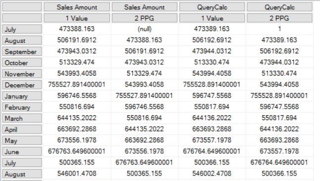
Here’s a query that includes a calculated measure defined in the WITH clause and returns two out of three of the members on the [Date Calc] dimension – but does not return the [3 YTD] calculation:

[sourcecode language=”text”]
WITH
MEMBER [Measures].QueryCalc AS
[Measures].[Sales Amount] + 1

SELECT
{
[Measures].[Sales Amount],
[Measures].QueryCalc
}
*
{
[Date Calc].[Date Calc].&[1 Value],
[Date Calc].[Date Calc].&[2 PPG]
}
ON 0,
[Date].[Calendar].[Month].MEMBERS
ON 1
FROM
TEST
[/sourcecode]

image

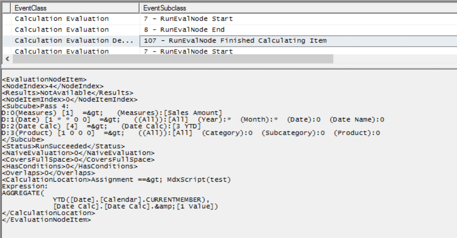
Running a Profiler trace as described in my previous post reveals that when this query is run, not only are the [Query Calc] and [2 PPG] calculations evaluated, but [3 YTD] is evaluated too:

image

It’s worth pointing out that this query was constructed deliberately to show a scenario where SSAS does decide to evaluate the [3 YTD] calculation, but in other cases it may decide otherwise. The reason it decides to do so here is due to a number of factors, including prefetching – see Jeffrey’s blog post here and the section on “Unexpected partition scans” here for some background information on this topic. Remember that in most cases prefetching is a good thing and is beneficial for performance, so if you see something like this happening in your cube you need to be sure that it’s actually causing you a performance problem before you try to prevent it.

If this is a problem for you there are a few things you can do. Rewriting your query to use subselects (if you have control over the MDX query that is being used) is one option:

[sourcecode language=”text”]
WITH
MEMBER [Measures].QueryCalc AS
[Measures].[Sales Amount] + 1

SELECT
{
[Measures].[Sales Amount],
[Measures].QueryCalc
}
*
{
[Date Calc].[Date Calc].MEMBERS
}
ON 0,
[Date].[Calendar].[Month].MEMBERS
ON 1
FROM
(SELECT
{
[Date Calc].[Date Calc].&[1 Value],
[Date Calc].[Date Calc].&[2 PPG]
}
ON 0
FROM
TEST)
CELL PROPERTIES VALUE
[/sourcecode]

Using the following connection string properties also works, because it turns off prefetching:

[sourcecode language=”text”]
disable prefetch facts=true; cache ratio=1
[/sourcecode]

…but as I said, this might hurt query performance in other ways.

Finally, as I said, using calculated members on your Date Tool dimension instead of the real members/scope statements approach will also work too. In my opinion this is the best solution since the problems with calculated member selection in Excel that caused problems for the calculated member Date Tool approach in the past were fixed a long time ago, and it will work even if you can’t change how your MDX queries are generated.

Finding Out Which MDX Calculations Are Being Evaluated By Your Query In Analysis Services Multidimensional, Part 1

Since Analysis Services 2012 there have been two trace events that provide a lot of information about what’s going on in the Formula Engine when you run a query in Analysis Services Multidimensional: Calculation Evaluation and Calculation Evaluation Detailed Information. The problem is that they are not properly documented anywhere and they provide so much information that it’s difficult to interpret what they are telling you. This post on Thomas Ivarrsson’s blog (which I strongly advise you to read before you carry on) with information provided by Akshai Mirchandani of the dev team  is the only place that has any details about them and unfortunately it’s by no means comprehensive.

I don’t have the knowledge to provide a full description of these two trace events, so instead in this series of posts I want to do something less ambitious but hopefully still useful: show how you can use them to find out which MDX calculations are being evaluated when you run a query, which is of course going to be useful if you are trying to tune that query. It’s not always as easy as you might think to work out which calculations are referenced by a query: for example financial cubes often have hundreds of calculated members and/or scoped assignments, many of which are dependent on other calculations.

Here’s a super-simple example to start off with. Imagine you have a cube with just one regular measure, Sales Amount, and just one calculated measure with the following definition:

[sourcecode language='text'  padlinenumbers='true']
CREATE MEMBER 
CURRENTCUBE.MEASURES.[Sales Forecast] AS
[Measures].[Sales Amount] * 2;
[/sourcecode]

Now, consider the following query:

[sourcecode language='text' ]
WITH
MEMBER MEASURES.X as 123
SELECT
{[Measures].[Sales Forecast]}
ON 0
,
[Date].[Date].[Date].MEMBERS
ON 1
FROM
[test]
CELL PROPERTIES VALUE
[/sourcecode]

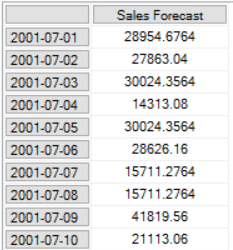
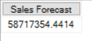
image

The query returns the Sales Forecast calculated measure on columns and every member on the Date level of the Date hierarchy on rows – so not all that interesting. However there are two things to point out:

  • The WITH clause has a calculated measure that isn’t used in the query. The reason I’ve put this in the query is to stop the Formula Engine from caching the results of any MDX calculations for longer than the lifetime of the query (see here for more details); it doesn’t affect the Storage Engine cache however. This means that every time the query is run you know that all the calculations will be evaluated and that you’ll be able to see any related activity in Profiler, and that you can run the query on a warm Storage Engine cache and won’t see many Storage Engine-related events.
  • The CELL PROPERTIES clause only returns the VALUE property and not the FORMAT_STRING property which is normally returned as well. This reduces the number of Calculation Evaluation events that are raised in Profiler when the query runs and makes it easier to see the important information.

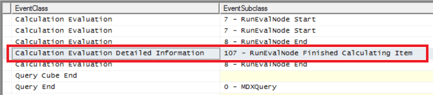
With a Profiler trace that includes the Calculation Evaluation and Calculation Evaluation Detailed Information events, when you run the query above you’ll see this:

image

There are a lot of events generated in the trace even for this simple query, but the important thing to look for is the line highlighted in the screenshot above: a Calculation Evaluation Detailed Information event with the following event subclass:

107 – RunEvalNode Finished Calculating Item

Any time you see this event you know that a calculation has been evaluated in bulk mode for a subcube (ie an area of cells) in your cube. You may see more than one RunEvalNode event for the same calculation in the same query if it was evaluated for more than one subcube.

The contents of the TextData column (which is displayed in the lower half of the screen in Profiler) for the RunEvalNode event in the trace shown above are as follows:

image

As you can see, it tells you the MDX expression that has been evaluated for the subcube. It also tells you the name of the calculated measure, but it’s the MDX expression that’s important here because scoped assignments that overlap with a single calculated measure could mean that many different MDX expressions must be evaluated for that calculated measure.

Now for the bad news: you won’t see a RunEvalNode event for any calculations that are evaluated in cell-by-cell mode. You probably know that inefficient or badly-written calculations are often evaluated in cell-by-cell mode, which is usually slower than bulk mode, but there are cases where the Formula Engine evaluates a perfectly good calculation in cell-by-cell mode because it’s the right thing to do. For example, take a look at the following query:

[sourcecode language='text' ]
WITH
MEMBER MEASURES.X as 123
SELECT
{[Measures].[Sales Forecast]}
ON 0
FROM
[test]
CELL PROPERTIES VALUE
[/sourcecode]


image

It’s basically the same query as the one above but with the Rows axis removed, so it only returns a single cell. In Profiler you won’t see a RunEvalNode event because in this case the Sales Forecast calculation is evaluated in cell-by-cell mode.

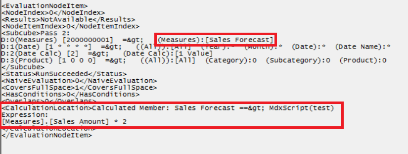
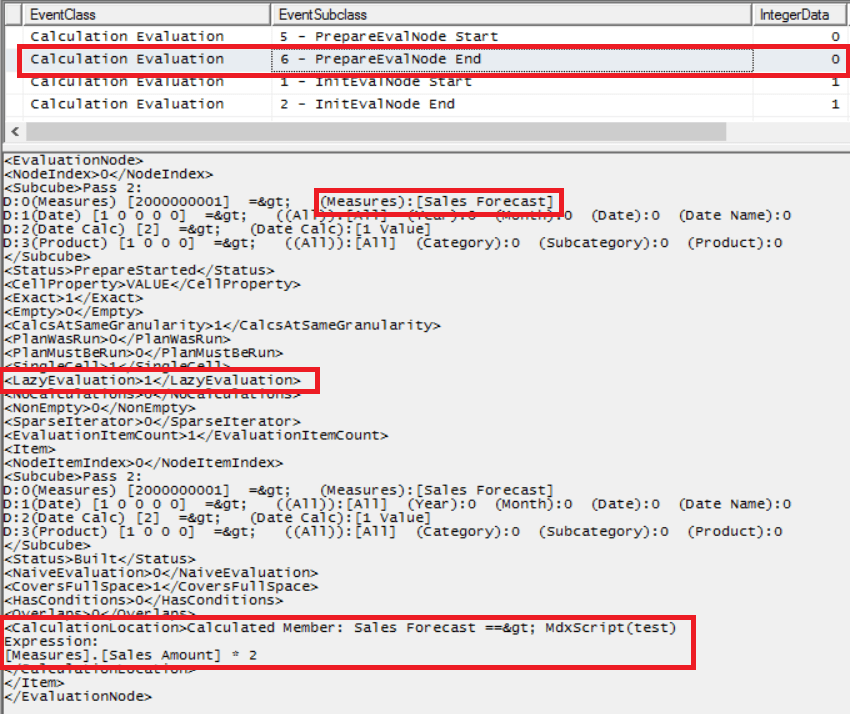
That said you will see other events relating to the evaluation node for the Sales Forecast calculation, such as the Calculation Evaluation event shown here, the last for this node (NodeIndex=0, the same value that is shown in the IntegerData column) in the trace:

image

Notice also the LazyEvaluation tag which is 1, which indicates a calculation that is evaluated in cell-by-cell mode.

So, to sum up, there are two ways to see which calculations are referenced by your query. With a Profiler trace and that includes the Calculation Evaluation and Calculation Evaluation Detailed Information events:

  1. If your calculation is evaluated in bulk mode you will see a Calculation Evaluation Detailed Information event with the Event Subclass 107 – RunEvalNode Finished Calculating Item.
  2. If your calculation is evaluated in cell-by-cell mode you will see Calculation Evaluation events for the Init-Build-Prepare stages of the evaluation node.

In the next post in this series I’ll look at a more complex scenario that shows some unexpected behaviour by SSAS.

[I am extremely grateful to Akshai Mirchandani for answering a lot of questions relating to this topic. If you want to learn more about the internals of the Formula Engine there are two other useful resources: this post by Jeffery Wang, also of the dev team, and chapter 29 of the book “Microsoft SQL Server 2008 Analysis Services Unleashed”]

The Show Hidden Cubes SSAS Connection String Property

If you need to write queries in SQL Server Management Studio against an SSAS cube that has its Visible property set to false, you have a problem because when you connect to your database you can’t see the cube or its metadata! Luckily you can override this and make the cube visible by setting the following connection string property when you connect:

Show Hidden Cubes=true

image

Connection string properties can be set in the Additional Connection Parameters tab of the connection dialog that appears when you open a new MDX query window.

Unfortunately this doesn’t make any objects in the cube that are not visible, like measures or dimensions, visible again – it just makes the cube itself visible. However, if you’re working on the Calculations tab of the Cube Editor in SSDT it is possible to make all hidden objects visible as I show here.

SSAS Documentation With Squarehouse Commentary

A few months ago I found out about a new tool for managing and viewing Analysis Services Multidimensional documentation called Squarehouse Commentary. I’ve now had the chance to play around with it and talk to the company that makes it and I have to say I’m impressed: in my opinion it’s by far the best tool of its type that I’ve seen. Rather than generating a large pile of documentation that no-one will read and which will get left, forgotten on a fileshare or a SharePoint site, it allows you to synch the descriptions created in its own web application with the description properties in your SSAS cubes and dimensions. It also automatically generates actions so that end users can easily view rich web-based documentation for hierarchies and measures direct from whatever client tool they are using in a few clicks.

This video does a good job of showing off the main features:

Overall, definitely something to check out. It doesn’t support Tabular models yet, but I’m told that this is in the planning stages.

SSAS Multidimensional Caching-Related Performance Problems With Power BI Tables

Last week I was doing some performance tuning for a customer using Power BI on top of a large SSAS Multidimensional cube via a Live connection. Some of their reports were performing particularly badly and I uncovered a problem with the DAX generated by Power BI for tables with a large number of rows, fields from two or more large hierarchies and totals turned on.

The problem is very easy to reproduce; I’m going to do it using a simplified version of the Adventure Works cube that contains only the Date and Product dimensions. Take a look at the following table from a Power BI report:

image

It has the Date attribute from the Date dimension, and the Product attribute from the Product dimension, on rows and two measures on columns. The table has a large number of rows in it (both Date and Product are fairly large hierarchies) and if you look at the DAX generated by Power BI you can see that it only requests the first 501 rows. That’s fine – the real problem is that Power BI also generates a second DAX query to get the two values displayed in the Total line at the bottom of the table. The DAX looks something like this, and is easily identifiable because it uses the Row() function:

[sourcecode language="text" padlinenumbers="true"]
EVALUATE
  CALCULATETABLE(
    ROW(
      "Sales_Amount", 'Internet Sales Facts'[Sales Amount],
      "Tax_Amt", 'Internet Sales Facts'[Tax Amt]
    ),
    KEEPFILTERS(
      GENERATE(
        KEEPFILTERS(VALUES('Product'[Product.Key0])),
        CALCULATETABLE(
          FILTER(
            KEEPFILTERS(VALUES('Order Date'[Date.Key0])),
            OR(
              NOT(ISBLANK('Internet Sales Facts'[Sales Amount])),
              NOT(ISBLANK('Internet Sales Facts'[Tax Amt]))
            )
          )
        )
      )
    )
  )
[/sourcecode]

This query has something in it – I don’t know what – that means that it cannot make use of the Analysis Services Storage Engine cache. Every time you run it SSAS will go to disk, read the data that it needs and then aggregate it, which means you’ll get cold-cache performance all the time. On a big cube this can be a big problem. This is very similar to problems I’ve seen with MDX queries on Multidimensional and which I blogged about here; it’s the first time I’ve seen this happen with a DAX query though. I suspect a lot of people using Power BI on SSAS Multidimensional will have this problem without realising it.

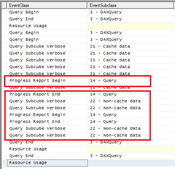
This problem does not occur for all tables – as far as I can see it only happens with tables that have a large number of rows and two or more hierarchies in. The easy way to check whether you have this problem is to refresh your report, run a Profiler trace that includes the Progress Report Begin/End and Query Subcube Verbose events (and any others you find useful) and then refresh the report again by pressing the Refresh button in Power BI Desktop without changing it at all. In your trace, if you see any of the Progress Report events appear when that second refresh happens, as well as Query Subcube Verbose events with an Event Subclass of Non-cache data, then you know that the Storage Engine cache is not being used.

image

Also look at the Duration column in the trace for these events which shows the time in milliseconds that they took to execute. This will tell you how much of an impact this problem is having on your report refresh times.

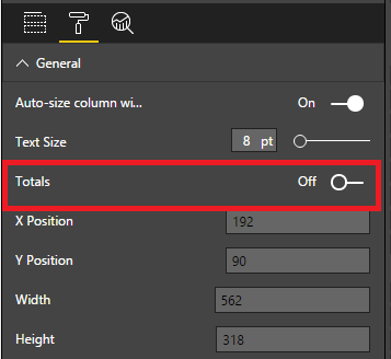
The easy way to stop this happening is to turn off the totals row in the table:

image

Displaying the totals in a separate table also seems to avoid the problem, although of course it doesn’t look as good. Only putting one hierarchy in the table apart from your measures, also seems to solve the problem. You could also try all the usual methods to improve SSAS performance such as building aggregations on the cube.

The dev team is aware of this problem but it’s unlikely to be fixed in the short term.

UPDATE 8th September 2020: This problem has finally been fixed as part of the general SuperDAX performance improvements in Analysis Services 2019 CU5. See https://powerbi.microsoft.com/en-us/blog/improving-power-bi-performance-when-querying-multidimensional-models/ for more details.

Deprecated And Discontinued Functionality In SSAS 2016

Some time ago I blogged about the deprecated and discontinued functionality in SSAS 2014, so I thought it would be a good idea to follow my last post on what’s new in SSAS 2016 Multidimensional with a discussion of what’s going or gone from it.

The same page that I linked to last time has been updated for 2016, and there are four more subpages with all the details. There’s nothing much interesting to say about the breaking changes (basically AMO has been rejigged) or behaviour changes (there’s no in-place upgrade for Tabular models using DirectQuery – you have to open the project and edit some settings) but the other two pages do have some news worthy of comment:

Discontinued Functionality

Here’s the official definition of a discontinued feature:

A discontinued feature is one that is no longer supported. It might also be physically removed from the product.

A few comments about what is now discontinued:

  1. The Non_Empty_Behavior property for calculated measures. To be honest, I’m happy to see this go: it doesn’t usually make much difference to performance and in most cases people use it incorrectly too. It really should be removed from Form View in the SSDT cube editor.
  2. COM assemblies. Note that this is not the same thing as .NET assemblies like the Analysis Services Stored Procedure Project! If you are using a custom MDX function implemented in a COM assembly you will probably find that the equivalent function implemented in a .NET assembly is a lot slower, but in my experience it’s almost always possible to avoid custom functions completely and use pure MDX – and this will give you the best query performance.
  3. I’m a bit sad to see the CalculationCurrentPass() and CalculationPassValue() functions die because you could do cool things like this with them, but I haven’t actually needed to use them for a long, long time.

Deprecated Functionality

Here’s the official definition of a deprecated feature:

A deprecated feature is a feature will be cut from the product in a future release, but is still supported and included in the current release to maintain backward compatibility. Typically, a deprecated feature is removed in a major release, often within two releases of the original announcement. For example, deprecated features announced in SQL Server 2012 are likely to be unsupported by SQL Server 2016.

A few comments on what’s been deprecated:

  1. The only thing that someone may possibly be using on the list of features that will not be supported in the next major release is linked dimensions; remote partitions and remote linked dimensions were always a very bad idea.
  2. The death of dimension writeback (note: not the same thing as writing values back to cells) is a bit of a shame: I never needed to use it, and most client tools didn’t support it, but it always struck me as one of those features that people might have used more if they had known about it.
  3. I see session cubes (as used by Excel PivotTables’ grouping functionality) will not be supported in a future release, which is probably a good thing given all the problems they cause. However I bet there are a lot of Excel workbooks out there that will be affected when this does go.
  4. Local cubes will also go in a future release, though I doubt anyone uses them anymore. That said, I think it would be really useful if there was something similar that allows you to create a Power Pivot model that was a local copy of an SSAS Tabular database, with the option to filter the data in it. Offline access is not so important these days but this would allow users to create their own customised Power Pivot models from a properly designed, central model rather than always having to start from scratch.
  5. Profiler for trace capture is also deprecated, and I discussed this in-depth here.


What’s New In Analysis Services 2016 Multidimensional?

With the recent release of SQL Server 2016 some of you old faithful SSAS Multidimensional users out there might be wondering if it’s worth upgrading. There is an official page describing what’s new in Analysis Services 2016 here:

https://msdn.microsoft.com/en-us/library/bb522628.aspx

…but it’s mostly concerned with SSAS Tabular and, unfortunately, it’s somewhat misleading. For example, it says:

a number of enhancements have been made to multidimensional models; for example, distinct count ROLAP optimization for data sources like DB2 and Oracle, drill-through multi-selection support with Excel 2016, and Excel query optimizations.

In fact the drillthrough/multi-select improvements (which I blogged about here) already shipped as part of SSAS 2014 and are reliant on improvements in Excel 2016 as much as in SSAS; similarly the Excel 2016 query optimisations are not reliant on any changes in SSAS 2016 and will benefit users of all versions of SSAS.

So what has actually changed with SSAS 2016 Multidimensional? I don’t know all the details on every change, but here’s what I know right now:

  • As the above quote shows, there have been improvements in ROLAP distinct count performance for DB2 and Oracle. I’ve also heard there are improvements for the SQL generated in ROLAP mode to take advantage of SQL Server’s columnstore indexes.
  • We now have Database Consistency Checker for SSAS, which you can read more about here or in Dustin Ryan’s post here. For Multidimensional it will only tell you whether your partition indexes are corrupt (it does a lot more for Tabular) and if they are you need to delete the database and then either restore it or re-deploy/reprocess.
  • Extended Events for SSAS now have UI support in SQL Server Management Studio, although the UI still looks like it needs some work. I still see myself using Profiler for my SSAS performance tuning work for the foreseeable future – or at least until I work out what the extra information that Extended Events give you is useful for. I know other people, like Bill Anton, are more excited about Extended Events and their possibilities though.
  • You can now use computer accounts to be members of the Analysis Services Administrators group in SQL Server Management Studio.
  • If you are developing applications that need to create, alter, process or otherwise do stuff to an Analysis Services database in .NET code then you need to be aware that Analysis Management Objects (AMO) has been refactored to include a second assembly which “paves the way for future extensions to AMO, with clear division between generic and context-specific APIs”.
  • There’s a new default setting for the MemoryHeapType server property that helps to avoid memory fragmentation and is relevant to Tabular and Multidimensional; Marco Russo has the details here.

Not the most exciting or inspiring set of changes, I have to say, even if there’s lots of cool new stuff in SSAS Tabular 2016. There are also usually other fixes and improvements like the MemoryHeapType property that get added but are never documented, and when I find out about them I’ll be sure to blog or tweet. If you find any please let me know!

Excel 2016 PivotTable MDX Changes Lead To Big Query Performance Gains

Yesterday, the Excel team announced a bunch of performance improvements in Excel 2016 for PivotTables connected to Analysis Services (Multidimensional or Tabular), Power Pivot and Power BI. If you haven’t read the official blog post already, here it is:

https://blogs.office.com/2016/07/07/faster-olap-pivottables-in-excel-2016/

In that post, Microsoft point out that how much of a performance increase you get will depend on a number of factors. I guess they have to do this to manage expectations. However I’m going to come right out and say that these changes are probably the most important thing that has happened in the last five years for Analysis Services or Power Pivot query performance and if you are using Excel PivotTables with SSAS or Power Pivot for reporting, you should upgrade to Excel 2016 (you’ll need the Office 365 click-to-run version) just for these changes.

The key improvement that Microsoft have made here is to stop Excel bringing back unnecessary subtotal values in the MDX queries that it generates. This has been a gigantic problem for years and several people have blogged about it: I did here, and among other people Rui Quintino and Richard Lees have posts on the subject that are worth reading. A lot of my consultancy work involves SSAS and MDX performance tuning and I think I see around five to ten customers every year who are seriously affected by this – and I’m sure this is just the tip of the iceberg. Even if you don’t think you are affected, you may have users who are putting up with slow refresh times for Excel-based reports without your knowledge.

Let’s go into some technical detail, see what the original problem was and what has changed in Excel 2016. I’m going to provide some examples using Excel 2013/2016 against SSAS Multidimensional but as I said the same problems occur (although less severely) with SSAS Tabular and Power Pivot.

Consider the following Excel 2013 PivotTable connected to the Adventure Works cube:

image
image

It’s typical of the kind of thing an end user wants to build, and there are two things to point out:

  1. Notice there are three fields that have been placed on the Rows axis of the PivotTable: the Gender and Marital Status hierarchies from the Customer dimension, and the Category hierarchy from the Product dimension. It’s pretty common for users to put many more fields together on an axis when they want to display detailed data.
  2. The user has also turned off grand totals and subtotals in the PivotTable so that only the detailed data is shown. This often happens in combination with (1) because if the user only wants to see the detailed data the subtotals and grand totals are a distraction.

In this case the PivotTable layout has been switched Tabular and the Repeat All Item Labels option is selected to make the PivotTable look like a table, but these are just aesthetic changes.

This PivotTable contains 12 rows, but if you look at the MDX query that is generated by Excel 2013 to populate it, it returns 36 rows of data (actually the MDX in this case returns 36 columns, but that’s a quirk of Excel) because the subtotals and grand total that Excel is not displaying are still being returned. Here’s the query:

SELECT 
NON EMPTY 
CrossJoin(
CrossJoin(
Hierarchize(
{DrilldownLevel(
{[Customer].[Gender].[All Customers]}
,,,INCLUDE_CALC_MEMBERS)}), 
Hierarchize(
{DrilldownLevel({[Customer].[Marital Status].[All Customers]}
,,,INCLUDE_CALC_MEMBERS)})), 
Hierarchize(
{DrilldownLevel({[Product].[Category].[All Products]}
,,,INCLUDE_CALC_MEMBERS)})) 
DIMENSION PROPERTIES PARENT_UNIQUE_NAME,HIERARCHY_UNIQUE_NAME 
ON COLUMNS  
FROM 
[Adventure Works] 
WHERE ([Measures].[Internet Sales Amount]) 
CELL PROPERTIES VALUE, FORMAT_STRING, 
LANGUAGE, BACK_COLOR, FORE_COLOR, FONT_FLAGS

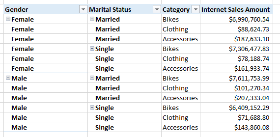
And here’s a sample of what it returns, with the unwanted values highlighted:

image

You can probably guess that these unwanted subtotals and grand totals make the query slower, and the more fields you put together on the rows or columns of a PivotTable the greater the number of subtotals/grand totals are returned and slower things get. PivotTables connected to SSAS or Power Pivot often become completely unusable with more than six or seven fields put together on the same axis, and the only workarounds before Excel 2016 are either to write custom MDX in a named set (I show how to do this here) or if you are using SSAS Multidimensional try to use member properties instead of separate fields (as Richard Lees shows here), but neither are really great alternatives.

Building the same PivotTable using Excel 2016, however, gives the following MDX:

SELECT 
NON EMPTY 
CrossJoin(
CrossJoin(
Hierarchize(
{[Customer].[Gender].[Gender].AllMembers}), 
Hierarchize(
{[Customer].[Marital Status].[Marital Status].AllMembers})), 
Hierarchize(
{[Product].[Category].[Category].AllMembers})) 
DIMENSION PROPERTIES PARENT_UNIQUE_NAME,HIERARCHY_UNIQUE_NAME 
ON COLUMNS  FROM [Adventure Works] 
WHERE ([Measures].[Internet Sales Amount]) 
CELL PROPERTIES VALUE, FORMAT_STRING, 
LANGUAGE, BACK_COLOR, FORE_COLOR, FONT_FLAGS

Which returns just the data needed for the PivotTable:

image

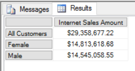
What has changed? Focusing on just the Gender hierarchy, the difference between the two queries is that in Excel 2013 the selection on Gender is given using the DrillDownLevel() function on the All Member of the hierarchy. Isolated and put in its own query, the set expression used looks like this:

SELECT 
{[Measures].[Internet Sales Amount]}
ON COLUMNS,
DrilldownLevel(
{[Customer].[Gender].[All Customers]}
,,,INCLUDE_CALC_MEMBERS)
ON ROWS
FROM
[Adventure Works]
image

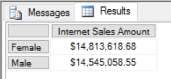
Notice how the All Member, used by Excel to return subtotals and grand totals, is returned by the set. Excel 2016 instead just asks for the members on the Gender level of the Gender hierarchy, not including the All Member. Again, put inside its own query, you can see what it returns:

SELECT 
{[Measures].[Internet Sales Amount]}
ON COLUMNS,
{[Customer].[Gender].[Gender].AllMembers}
ON ROWS
FROM
[Adventure Works]
image

Apart from the fact that no All Member is returned, it’s also a lot cleaner and easier to read.

I’ve been very excited about this change since I first heard it was happening, and I think it will benefit a lot of people. A big thanks to Alexander Lahuerta and the rest of the Excel team for making this happen!