Using the Resource Usage Profiler Event For SSAS Multidimensional Query Performance Tuning, Part 1: Rows Scanned And Rows Returned

If you’re performance tuning SSAS Multidimensional Storage Engine issues, the Resource Usage Profiler event can provide a lot of useful information about what’s going on behind the scenes when you run a query. This is something I have blogged about in the past (and it will be useful to read this post before carrying on) but recently I’ve done some more research into this area and found out a lot more things about what this event tells you.

For my testing I created a very simple cube from a single fact table. The table contained 5000 rows and two columns: a dimension key column containing the values 1 to 5000, and a measure column that always contained the value 1. From this I built a single measure group with a single measure called My Measure, and a single dimension built from the dimension key column with 5000 members on it called ID.

Consider the following MDX query:

[sourcecode language=”text” padlinenumbers=”true”]
SELECT
{[Measures].[My Measure]}
ON 0
FROM
[MyCube]
WHERE([ID].[ID].&[1])
[/sourcecode]

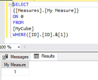
Here’s the output:

image

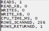
In this query the WHERE clause filters the output to one member from the ID dimension, which in turn returns data from one row in the underlying fact table, and so My Measure returns 1. If the query is run on cold cache, the Resource Usage Profiler event returns the following:

image

The ROWS_RETURNED value here returns 1, which is what you might expect – the query results show data from one row in the underlying fact table. The ROWS_SCANNED value is 256 though. Why? Chapter 20 of the book “Microsoft SQL Server 2008 Analysis Services Unleashed” has a lot of detail about how SSAS MD stores data on disk, but the important point here is that the data in a partition is stored on disk in segments, with each segment made up of pages, and when a query is run SSAS will scan all the pages that it thinks contain data. The ever-reliable Akshai Mirchandani of the SSAS dev team helped me with the remaining information I needed:

  • There are 65536 rows of data per segment
  • There are 256 pages per segment
  • There are therefore, at most, 256 rows per page

So in this case ROWS_SCANNED shows 256 because one complete page was scanned.

Modifying the query to slice on two members from ID like so:

[sourcecode language=”text”]
SELECT
{[Measures].[My Measure]}
ON 0
FROM
[MyCube]
WHERE([ID].[ID].&[1]:[ID].[ID].&[2])
[/sourcecode]

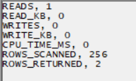
image

…results in a ROWS_RETURNED of 2 and a ROWS_SCANNED that is still 256, because the two rows must be stored in the same page:

image

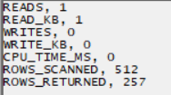
…while asking for 257 members from ID in the WHERE clause like so:

[sourcecode language=”text”]
SELECT
{[Measures].[My Measure]}
ON 0
FROM
[MyCube]
WHERE([ID].[ID].&[1]:[ID].[ID].&[257])
[/sourcecode]

Results in a ROWS_RETURNED of 257 and a ROWS_SCANNED of 257 – obviously 2 pages are now being scanned to get the data needed for the query.

image

Finally, the query:

[sourcecode language=”text” padlinenumbers=”true”]
SELECT
{[Measures].[My Measure]}
ON 0
FROM
[MyCube]
WHERE([ID].[ID].&[5000])
[/sourcecode]

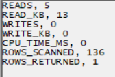
…returns a rows scanned of 136:

image

This must be because the final page, which doesn’t contain the full 256 rows, is scanned. 5000-136=4864, and 4864/256=19, so there must be 20 pages of data: 19 pages of 256 rows and one final page of 136 rows.

I don’t think it’s worth getting too hung up on the exact values that ROWS_SCANNED and ROWS_RETURNED, especially given that they return totals for all Storage Engine activity for all measure groups for the whole query, but knowing that they tell you roughly how much work is being done my the Storage Engine means that you can use them to watch for warning signs that something isn’t working properly when you’re performance tuning queries. In subsequent parts of this series I’ll show some practical examples of this.

Drillthrough On Calculated Members In SSAS MD 2017 Using DAX Expressions, Part 2

If you read part 1 of this series you probably already have a good idea of how I’m going to use DAX queries in actions to implement drillthrough on calculated members. However, there is one last major problem to solve – and no 100% fool-proof way of solving it.

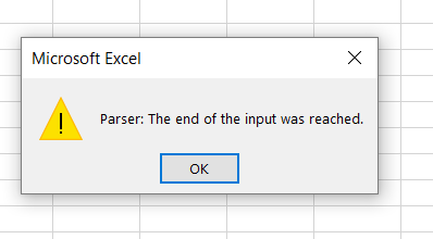
That problem is that there is a maximum length of (as far as I can tell) 32768 characters for the DAX query that is generated by the action. If you exceed that limit you’ll see an error in Excel when you drillthrough:

image

This is the result of the generated DAX query being truncated before Excel tries to run it. As you can imagine, if you have large dimensions and you’re generating a DAX query with thousands of key values in an IN expression, it’s very easy to hit the maximum query length. What can you do to make this less likely?

Probably the most effective method is to check whether the IN clause will contain all of the possible key values on the dimension (most likely because no attributes from the dimension are used in the query), and if so don’t bother including that dimension in the DAX query. Here’s an example of how this can be done:

[sourcecode language=”text” padlinenumbers=”true”]
IIF(
COUNT(EXISTING [Date].[Date].[Date].MEMBERS) =
COUNT([Date].[Date].[Date].MEMBERS),
"",
",’Date'[Date.Key0] IN {
" +
GENERATE(EXISTING [Date].[Date].[Date].MEMBERS ,
[Date].[Date].CURRENTMEMBER.PROPERTIES("KEY"), ",")
+ "}
")
[/sourcecode]

Another option is to use NonEmpty() to remove any members from the drillthrough that have no data, like so:

[sourcecode language=”text” highlight=”8″]
IIF(
COUNT(EXISTING [Date].[Date].[Date].MEMBERS) =
COUNT([Date].[Date].[Date].MEMBERS),
"",
",’Date'[Date.Key0] IN {
" +
GENERATE(EXISTING
NONEMPTY([Date].[Date].[Date].MEMBERS, [Measures].[Sales Amount])
, [Date].[Date].CURRENTMEMBER.PROPERTIES("KEY"), ",")
+ "}
")
[/sourcecode]

However, if these techniques (and there may be others) still don’t reduce the length of the query to an acceptable length you will want to try to fail as gracefully as possible and show a more helpful error message than the one above. You can do this with the DAX Error() function, like so:

[sourcecode language=”text”]
IIF(
COUNT(EXISTING [Customer].[Customer].[Customer].MEMBERS) =
COUNT([Customer].[Customer].[Customer].MEMBERS),
"",
",’Customer'[Customer.Key0] IN {
" +
IIF(COUNT(
{EXISTING
NONEMPTY(
[Customer].[Customer].[Customer].MEMBERS,
[Measures].[Sales Amount])}
AS CustomerList)>7000,
"ERROR(
""Please reduce your selection on the Customer dimension
or remove it from your PivotTable"")",
GENERATE(
CustomerList
, [Customer].[Customer].CURRENTMEMBER.PROPERTIES("KEY"), ",")
)
+ "}
")
[/sourcecode]

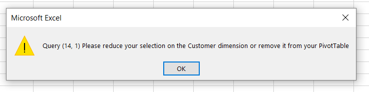
In this example, if the resulting DAX IN expression for the Customer dimension will have more than 7000 keys in it, the entire DAX query returns a custom error message instead:

image

Once again this is a far from perfect solution – I would have liked to test the total number of characters in the query, but if you do that you have to write the expression twice, once in the first parameter of IIF() and once in one of the results, and that would be horrible. My gut feeling is that you should only use this technique on dimensions with a large number of members on the key attribute.

Putting this all together, for a simple cube based on data from Adventure Works with three dimensions (Date, Product and Customer) here’s what a complete Action Expression for a regular measure might look like:

[sourcecode language=”text” padlinenumbers=”true”]
"EVALUATE
FILTER(
CALCULATETABLE(
SELECTCOLUMNS(
‘Sales Order’,
""Sales Order Number"",
‘Sales Order'[Sales Order Number],
""Sales Order Line Number"",
‘Sales Order'[Sales Order Line Number],
""Sales Amount"",
[Sales Amount])
" +
IIF(
COUNT(EXISTING [Date].[Date].[Date].MEMBERS) =
COUNT([Date].[Date].[Date].MEMBERS),
"",
",’Date'[Date.Key0] IN {
" +
GENERATE(EXISTING
NONEMPTY([Date].[Date].[Date].MEMBERS,
[Measures].[Sales Amount])
, [Date].[Date].CURRENTMEMBER.PROPERTIES("KEY"), ",")
+ "}
") +
IIF(
COUNT(EXISTING [Customer].[Customer].[Customer].MEMBERS) =
COUNT([Customer].[Customer].[Customer].MEMBERS),
"",
",’Customer'[Customer.Key0] IN {
" +
IIF(
COUNT(
{EXISTING NONEMPTY([Customer].[Customer].[Customer].MEMBERS,
[Measures].[Sales Amount])} AS CustomerList)>7000,
"ERROR(""Please reduce your selection on the Customer dimension
or remove it from your PivotTable"")",
GENERATE(
CustomerList
, [Customer].[Customer].CURRENTMEMBER.PROPERTIES("KEY"), ",")
)
+ "}
") +
IIF(
COUNT(EXISTING [Product].[Product].[Product].MEMBERS) =
COUNT([Product].[Product].[Product].MEMBERS),
"",
",’Product'[Product.Key0] IN {
" +
GENERATE(EXISTING
NONEMPTY([Product].[Product].[Product].MEMBERS,
[Measures].[Sales Amount])
, [Product].[Product].CURRENTMEMBER.PROPERTIES("KEY"), ",")
+ "}
") +
"),
[Sales Amount]>0)"
[/sourcecode]


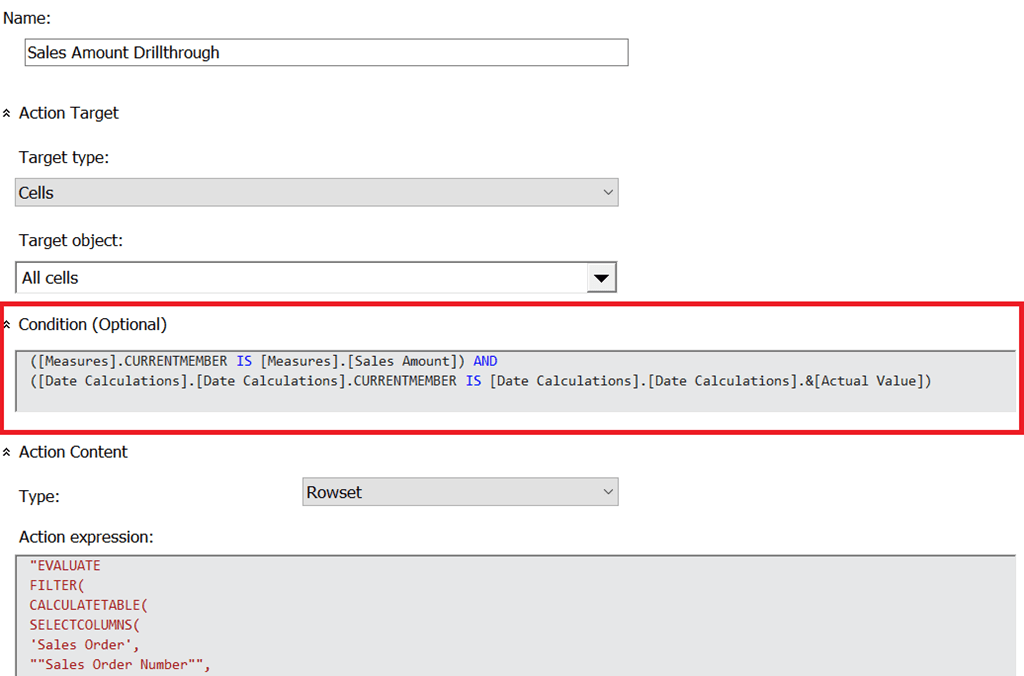
What about a calculated measure though? Assuming that  you have a time utility/date tool/shell dimension, you can use a Condition expression on the action above to make sure it only gets executed for the member on the time utility dimension that contains the non-calculated values, in this case called [Actual Value]:

[sourcecode language=”text”]
([Measures].CURRENTMEMBER IS [Measures].[Sales Amount]) AND
([Date Calculations].[Date Calculations].CURRENTMEMBER IS
[Date Calculations].[Date Calculations].&[Actual Value])
[/sourcecode]

image

Now, let’s say there is a calculated member on the time utility dimension that contains a year-to-date calculation with the following definition:

[sourcecode language=”text”]
CREATE MEMBER
CURRENTCUBE.[Date Calculations].[Date Calculations].[Year-To-Date]
AS
AGGREGATE(
PERIODSTODATE(
[Date].[Calendar].[Year],
[Date].[Calendar].CURRENTMEMBER),
[Date Calculations].[Date Calculations].&[Actual Value]);
[/sourcecode]

You can create a new action that has a Condition expression as follows that restricts it to the year-to-date calculation:

[sourcecode language=”text”]
([Measures].CURRENTMEMBER IS [Measures].[Sales Amount]) AND
([Date Calculations].[Date Calculations].CURRENTMEMBER IS
[Date Calculations].[Date Calculations].[Year-To-Date])
[/sourcecode]

Now, the final problem to solve is to generate a DAX query that returns all of the Sales Orders from the beginning of the current year up to and including the selected date – the Sales Orders that a user would expect to see when they drilled through on the year-to-date calculated member above.

Here’s a modified MDX expression for the Date dimension that returns a DAX expression that finds all of the dates associated with the current selection on the Date dimension, finds the maximum date, then filters the drillthrough DAX query by all dates from the beginning of the current calendar year up to and including the maximum date:

[sourcecode language=”text”]
IIF(
COUNT(EXISTING [Date].[Date].[Date].MEMBERS) =
COUNT([Date].[Date].[Date].MEMBERS),
"",
", VAR FilteredDates = FILTER(‘Date’, ‘Date'[Date.Key0] IN {
" +
GENERATE(
EXISTING
NONEMPTY([Date].[Date].[Date].MEMBERS,[Measures].[Sales Amount]) ,
[Date].[Date].CURRENTMEMBER.PROPERTIES("KEY"), ",")
+ "})
VAR MaxDate = MAXX(FilteredDates, ‘Date'[Date.Key0])
VAR MaxYear = MAXX(FilteredDates, ‘Date'[Year])
RETURN
FILTER(‘Date’, ‘Date'[Date.Key0]<=MaxDate && ‘Date'[Year]=MaxYear)
")
[/sourcecode]

Here’s the complete MDX expression for the year-to-date drillthrough:

[sourcecode language=”text”]
"EVALUATE
FILTER(
CALCULATETABLE(
SELECTCOLUMNS(
‘Sales Order’,
""Sales Order Number"",
‘Sales Order'[Sales Order Number],
""Sales Order Line Number"",
‘Sales Order'[Sales Order Line Number],
""Sales Amount"",
[Sales Amount])
" +
IIF(
COUNT(EXISTING [Date].[Date].[Date].MEMBERS) =
COUNT([Date].[Date].[Date].MEMBERS),
"",
", VAR FilteredDates = FILTER(‘Date’, ‘Date'[Date.Key0] IN {
" +
GENERATE(
EXISTING
NONEMPTY([Date].[Date].[Date].MEMBERS,[Measures].[Sales Amount]) ,
[Date].[Date].CURRENTMEMBER.PROPERTIES("KEY"), ",")
+ "})
VAR MaxDate = MAXX(FilteredDates, ‘Date'[Date.Key0])
VAR MaxYear = MAXX(FilteredDates, ‘Date'[Year])
RETURN
FILTER(‘Date’, ‘Date'[Date.Key0]<=MaxDate && ‘Date'[Year]=MaxYear)
") +
IIF(
COUNT(EXISTING [Customer].[Customer].[Customer].MEMBERS) =
COUNT([Customer].[Customer].[Customer].MEMBERS),
"",
",’Customer'[Customer.Key0] IN {
" +
IIF(COUNT({
EXISTING
NONEMPTY([Customer].[Customer].[Customer].MEMBERS,
[Measures].[Sales Amount])} AS CustomerList)>7000,
"ERROR(""Please reduce your selection on the Customer dimension or
remove it from your PivotTable"")",
GENERATE(
CustomerList
, [Customer].[Customer].CURRENTMEMBER.PROPERTIES("KEY"), ",")
)
+ "}
") +
IIF(
COUNT(EXISTING [Product].[Product].[Product].MEMBERS) =
COUNT([Product].[Product].[Product].MEMBERS),
"",
",’Product'[Product.Key0] IN {
" +
GENERATE(EXISTING
NONEMPTY([Product].[Product].[Product].MEMBERS,
[Measures].[Sales Amount])
, [Product].[Product].CURRENTMEMBER.PROPERTIES("KEY"), ",")
+ "}
") +
"),
[Sales Amount]>0)"
[/sourcecode]

I warned you it was going to be complicated, didn’t I? You can download a SSAS MD 2017 .abf backup file containing the sample database and the two actions here.

SSAS Multidimensional HOLAP Storage: Even More Useless Than You Might Think

In almost 20 years of using Analysis Services I have never, ever used HOLAP storage. However the other week I was with a customer that was using ROLAP storage on top of Exasol and while query performance was generally good, I wondered whether building an aggregation or two in SSAS might help query performance in some cases. Surely HOLAP could be useful here? Sadly not.

What I hadn’t realised was that when you use HOLAP storage and process a partition, SSAS generates exactly the same fact table-level SQL query that is used to process a MOLAP partition. It then uses this data to build any aggregations you have defined and after that throws the data it has read away, leaving only the aggregations stored in MOLAP mode. Therefore you get exactly the same, slow processing performance as pure MOLAP storage and worse query performance! It even executes the SQL query when there are no aggregations defined. I had assumed SSAS would generate one SQL query for each aggregation and get just the summarised data needed by the aggregation but I was wrong. This means that for the kind of scenarios where ROLAP on a fast relational database is becoming more popular (for example when working with large data volumes and/or real-time data) HOLAP is not a viable option.

Tuning MDX Calculations That Use The Root() Function

Something that I have vaguely known about for years (for example from Mosha’s post here), but somehow never blogged about, is that using the Root() function in MDX calculations is not great for performance. I’m pretty sure that someone once told me that it was intended for use with defining subcubes for SCOPE statements and not inside calculations at all, which maybe why it hasn’t been optimised. Anyway, here’s an example of the problem and how to work around it.

Take the following query on the Adventure Works cube:

[sourcecode language='text'  padlinenumbers='true' highlight='4']
WITH
MEMBER MEASURES.DEMO AS
([Measures].[Internet Sales Amount],
ROOT([Date]))

SELECT 
{[Measures].[Internet Sales Amount],
MEASURES.DEMO} 
ON 0,
NON EMPTY
[Date].[Calendar].[Calendar Year].MEMBERS
*
[Customer].[Customer].[Customer].MEMBERS
ON 1
FROM
[Adventure Works]
[/sourcecode]

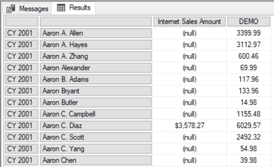
It returns sales for all customers by year, and the calculated measure returns the sales for each customer across all dates using the Root() function.

image

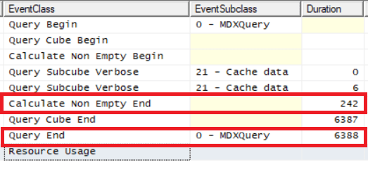
On a warm SE cache (which means the amount of time taken by the query will be dependent on how quickly SSAS can do the calculation and evaluate the Non Empty) on my laptop this takes a touch over 7 seconds:

image

Notice also that the Calculate Non Empty End event tells us that the Non Empty filter alone took 2.8 seconds (see here for some more detail on this event).

Now if you rewrite the query, replacing the Root() function with the All Member on the Calendar hierarchy like so:

[sourcecode language='text'  highlight='4']
WITH
MEMBER MEASURES.DEMO AS
([Measures].[Internet Sales Amount],
[Date].[Calendar].[All Periods])

SELECT 
{[Measures].[Internet Sales Amount],
MEASURES.DEMO} 
ON 0,
NON EMPTY
[Date].[Calendar].[Calendar Year].MEMBERS
*
[Customer].[Customer].[Customer].MEMBERS
ON 1
FROM
[Adventure Works]
[/sourcecode]

The query returns the same results, but in just over 5.5 seconds and with the Non Empty taking about 10% of the time it previously took.

image

I’m making a big assumption here though: the Root() function in the first query returns a tuple containing every All Member from every hierarchy on the Date dimension, not just the All Member from the Calendar hierarchy, so while these two queries return the same results the calculations are not equivalent. You can still get a performance improvement, though, by replacing the Root() function with the tuple it returns, although the resulting MDX will look very messy.

First, to find what the Root() function returns just use a query like this:

[sourcecode language='text' ]
WITH
MEMBER MEASURES.ROOTRETURNS as 
TUPLETOSTR(ROOT([Date]))
SELECT {MEASURES.ROOTRETURNS} ON 0
FROM
[Adventure Works]
[/sourcecode]

Run it in SQL Server Management Studio and you can copy/paste the tuple from the query results:

image

Here’s the tuple I get from my (somewhat hacked around) Date dimension:

[sourcecode language='text' ]
([Date].[Fiscal].[All Periods],[Date].[Calendar].[All Periods],[Date].[Calendar Weeks].[All Periods],
[Date].[Fiscal Weeks].[All Periods],[Date].[Fiscal Year].[All Periods],[Date].[Date].[All Periods],
[Date].[Calendar Quarter].[All Periods],[Date].[Fiscal Quarter].[All Periods],
[Date].[Calendar Semester].[All Periods],[Date].[Fiscal Semester].[All Periods],
[Date].[Day of Week].[All Periods],[Date].[Day Name].[All Periods],
[Date].[Day of Month].[All Periods],[Date].[Day of Year].[All Periods],
[Date].[Calendar Week].[All Periods],[Date].[Month Name].[All Periods],
[Date].[Calendar Year].[All Periods],[Date].[Fiscal Semester of Year].[All Periods],
[Date].[Calendar Semester of Year].[All Periods],[Date].[Fiscal Quarter of Year].[All Periods],
[Date].[Calendar Quarter of Year].[All Periods],[Date].[Month of Year].[All Periods],
[Date].[Fiscal Week].[All Periods],[Date].[Calendar Week of Year].[All Periods],
[Date].[Fiscal Week of Year].[All Periods],[Date].[Current Date].[All Periods],
[Date].[Is2002].[All Periods],[Date].[Month Day].[All Periods])
[/sourcecode]

Yuck. Anyway, with this gigantic tuple inserted into our calculation like so:

[sourcecode language='text'  highlight='4']
WITH
MEMBER MEASURES.DEMO AS
([Measures].[Internet Sales Amount],
[Date].[Fiscal].[All Periods],[Date].[Calendar].[All Periods],[Date].[Calendar Weeks].[All Periods],[Date].[Fiscal Weeks].[All Periods],[Date].[Fiscal Year].[All Periods],[Date].[Date].[All Periods],[Date].[Calendar Quarter].[All Periods],[Date].[Fiscal Quarter].[All Periods],[Date].[Calendar Semester].[All Periods],[Date].[Fiscal Semester].[All Periods],[Date].[Day of Week].[All Periods],[Date].[Day Name].[All Periods],[Date].[Day of Month].[All Periods],[Date].[Day of Year].[All Periods],[Date].[Calendar Week].[All Periods],[Date].[Month Name].[All Periods],[Date].[Calendar Year].[All Periods],[Date].[Fiscal Semester of Year].[All Periods],[Date].[Calendar Semester of Year].[All Periods],[Date].[Fiscal Quarter of Year].[All Periods],[Date].[Calendar Quarter of Year].[All Periods],[Date].[Month of Year].[All Periods],[Date].[Fiscal Week].[All Periods],[Date].[Calendar Week of Year].[All Periods],[Date].[Fiscal Week of Year].[All Periods],[Date].[Current Date].[All Periods],[Date].[Is2002].[All Periods],[Date].[Month Day].[All Periods])

SELECT 
{[Measures].[Internet Sales Amount],
MEASURES.DEMO} 
ON 0,
NON EMPTY
[Date].[Calendar].[Calendar Year].MEMBERS
*
[Customer].[Customer].[Customer].MEMBERS
ON 1
FROM
[Adventure Works]
[/sourcecode]

The query is a little slower – just over 6 seconds- but still faster than the first query using Root(), and the Non Empty filter is still fast:

image

Something else to watch out for with Root(), and another good reason not to use it in calculations, is that it returns an error in certain multiselect scenarios as Richard Lees describes here.

Obscure MDX Month: Optimising MDX That Uses The RGB() Function

In the first blog post in this series a few weeks ago I mentioned that calling Excel and VBA functions from MDX came with a query performance penalty. In this post I’ll give you an illustration of this using the VBA function that I suspect is most frequently called in MDX: the RGB() function.

Take the following MDX query as a baseline:

[sourcecode language=”text”]
WITH
MEMBER MEASURES.TEST AS
[Measures].[Internet Sales Amount]
SELECT {[Customer].[Country].[Country].MEMBERS} ON 0,
NON EMPTY
[Date].[Date].[Date].MEMBERS
*
[Product].[Product].[Product].MEMBERS
ON 1
FROM
[Adventure Works]
WHERE(MEASURES.TEST)
CELL PROPERTIES
VALUE,
FORMATTED_VALUE,
BACK_COLOR
[/sourcecode]


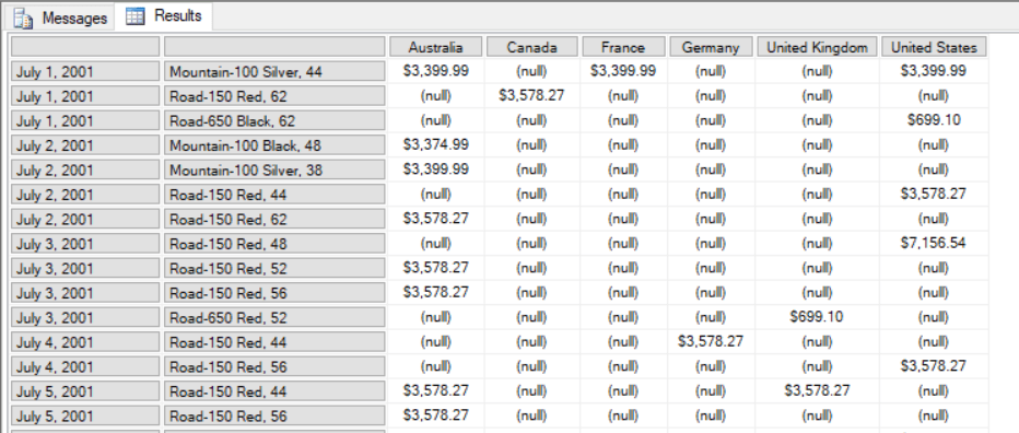
It returns Countries on columns and all non empty combinations of Date and Product on rows, and the calculated measure returns the value of the Internet Sales Amount measure:

image

On a SE engine cache it runs in 2.5 seconds on my laptop. With a BACK_COLOR property added to the calculated measure that uses the RGB() function to return the code for red if the measure value is greater than $5000, query performance is a lot worse: it goes up to 6.5 seconds on a warm SE cache.

[sourcecode language=”text” highlight=”4,5,6,7″]
WITH
MEMBER MEASURES.TEST AS
[Measures].[Internet Sales Amount]
,BACK_COLOR=
IIF([Measures].[Internet Sales Amount]>5000,
RGB(255,0,0),
RGB(255,255,255))
SELECT {[Customer].[Country].[Country].MEMBERS} ON 0,
NON EMPTY
[Date].[Date].[Date].MEMBERS
*
[Product].[Product].[Product].MEMBERS
ON 1
FROM
[Adventure Works]
WHERE(MEASURES.TEST)
CELL PROPERTIES VALUE, FORMATTED_VALUE, BACK_COLOR
[/sourcecode]


image

That’s a big increase just to do some cell highlighting! However in this case the RGB() function can only return two possible integer values, so if you replace the RGB() function with the integers it returns, like so:

[sourcecode language=”text” highlight=”4,5,6,7″]
WITH
MEMBER MEASURES.TEST AS
[Measures].[Internet Sales Amount]
,BACK_COLOR=
IIF([Measures].[Internet Sales Amount]>5000,
255,
16777215)
SELECT {[Customer].[Country].[Country].MEMBERS} ON 0,
NON EMPTY
[Date].[Date].[Date].MEMBERS
*
[Product].[Product].[Product].MEMBERS
ON 1
FROM
[Adventure Works]
WHERE(MEASURES.TEST)
CELL PROPERTIES VALUE, FORMATTED_VALUE, BACK_COLOR
[/sourcecode]

…then the query returns in around 3.5 seconds. The last thing to remember is that IIF() statements can perform better if one branch returns null, and in this case we can replace the integer value 16777215 that gives the white background with a null and get the same result:

[sourcecode language=”text” highlight=”4,5,6,7″]
WITH
MEMBER MEASURES.TEST AS
[Measures].[Internet Sales Amount]
,BACK_COLOR=
IIF([Measures].[Internet Sales Amount]>5000,
255,
16777215)
SELECT {[Customer].[Country].[Country].MEMBERS} ON 0,
NON EMPTY
[Date].[Date].[Date].MEMBERS
*
[Product].[Product].[Product].MEMBERS
ON 1
FROM
[Adventure Works]
WHERE(MEASURES.TEST)
CELL PROPERTIES VALUE, FORMATTED_VALUE, BACK_COLOR
[/sourcecode]

Now the query returns in around 3 seconds, only 0.5 seconds slower than the original with no colour coding.

Obscure MDX Month: Optimising The Performance Of Total-To-Date Calculations In SSAS Multidimensional

Here’s a SSAS Multidimensional MDX tip that I picked up at the PASS Summit back in 2008 at Mosha’s excellent “MDX Deep Dive” precon (incidentally the slides and supporting material are still available here, although a lot of the material is out of date). It’s regarding total-to-date calculations, ie calculations where you are doing a running total from the very first date you have data for up to the current date. The standard way of writing these calculations is something like this:

[sourcecode language='text'  padlinenumbers='true' highlight='3,4,5']
WITH
MEMBER MEASURES.[TTD Sales] AS
SUM(
NULL:[Date].[Calendar].CURRENTMEMBER,
[Measures].[Internet Sales Amount])

SELECT
[Customer].[Country].[Country].MEMBERS 
ON 0,
NON EMPTY
[Date].[Calendar].[Date].MEMBERS
*
[Product].[Product].[Product].MEMBERS
ON 1
FROM
[Adventure Works]
WHERE(MEASURES.[TTD Sales])
[/sourcecode]

This query runs in around 19.2 seconds on my laptop on a cold cache. However if you rewrite it like this:

[sourcecode language='text'  highlight='3,4,5,8,9,10,11,12,13']
WITH
MEMBER MEASURES.[PTTD SALES] AS
SUM(
NULL:[Date].[Calendar].CURRENTMEMBER.PARENT.PREVMEMBER,
[Measures].[Internet Sales Amount])

MEMBER MEASURES.[TTD Sales] AS
MEASURES.[PTTD SALES]
+
SUM(
[Date].[Calendar].CURRENTMEMBER.FIRSTSIBLING:
[Date].[Calendar].CURRENTMEMBER,
[Measures].[Internet Sales Amount])

SELECT
[Customer].[Country].[Country].MEMBERS 
ON 0,
NON EMPTY
[Date].[Calendar].[Date].MEMBERS
*
[Product].[Product].[Product].MEMBERS
ON 1
FROM
[Adventure Works]
WHERE(MEASURES.[TTD Sales])
[/sourcecode]

…it runs slightly faster: around 16.1 seconds on a cold cache on my laptop. Of course this is a very big query, and on most normal queries the difference in performance would be much less significant, but it could still be useful. In fact it’s very similar to the kind of tricks people used to optimise the performance of YTD calculations back in the days of SSAS 2000 – the subject of my second-ever blog post from December 2004! The idea here is that instead of summing up a large set of dates, the calculation sums up all the dates in the current month and then all the months from the beginning of time up to and including the previous full month. For YTD and most other something-to-date calculations trick like this are no longer needed, and indeed are counter-productive and will make your calculations slower. However it seems that for total-to-date calculations they can still help performance.

Obscure MDX Month: Current and CurrentOrdinal

When you are writing an MDX expression, everywhere you use a set you can give that set a name and then reference the name later on. This is known as creating an inline named set, something I have blogged about a few times (see here and here) over the years. When you are iterating over a set using a function like Generate() or Filter(), if you give that set a name you can then use the Current and CurrentOrdinal functions to find out more about the item in the set returned at the current iteration.

Consider the following MDX query on the Adventure Works cube:

[sourcecode language=”text”]
SELECT
{[Measures].[Internet Sales Amount]}
ON 0,
{[Customer].[Gender].[Gender].MEMBERS
*
[Customer].[Marital Status].[Marital Status].MEMBERS}
ON 1
FROM
[Adventure Works]
[/sourcecode]

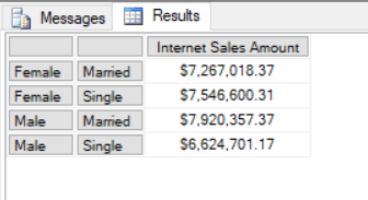
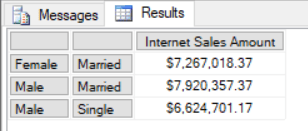
It returns a set of four tuples on rows: every combination of Gender and Marital Status:

image

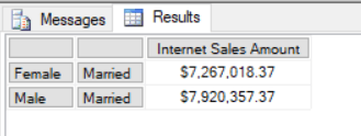
If you pass the set on rows to the Filter() function and give it a name (for example MySet) you can then use the CurrentOrdinal function to find the 1-based ordinal of the current iteration. This query uses the CurrentOrdinal function to filter the set shown above so only the first and third items in the set are returned:

[sourcecode language=”text”]
SELECT {[Measures].[Internet Sales Amount]} ON 0,
FILTER(
{[Customer].[Gender].[Gender].MEMBERS
*
[Customer].[Marital Status].[Marital Status].MEMBERS}
AS MYSET,
MYSET.CURRENTORDINAL=1 OR
MYSET.CURRENTORDINAL=3)
ON 1
FROM
[Adventure Works]
[/sourcecode]


image

With an inline named set you can also use the Current function to return the tuple at the current iteration. Here’s another query that uses the Current function to remove the tuple (Female, Single) from the set:

[sourcecode language=”text”]
SELECT
{[Measures].[Internet Sales Amount]} ON 0,
FILTER(
{[Customer].[Gender].[Gender].MEMBERS
*
[Customer].[Marital Status].[Marital Status].MEMBERS}
AS MYSET,
NOT(
MYSET.CURRENT IS
([Customer].[Gender].&[F],[Customer].[Marital Status].&[S])
)
)
ON 1
FROM
[Adventure Works]
[/sourcecode]

image

I won’t pretend that these functions are massively useful, but fans of super-complex MDX will enjoy this vintage post where I used them.

Obscure MDX Month: Recreating The Star Ratings Measure In MDX Using Excel Functions

I still love MDX, but I’m aware that I blog about it less and less – which is a shame, I know. Therefore I’ve decided that for the next four weeks I’m going to write about some obscure MDX topics that hopefully will make all you SSAS MD diehards out there feel less neglected… even if they don’t have much practical use.

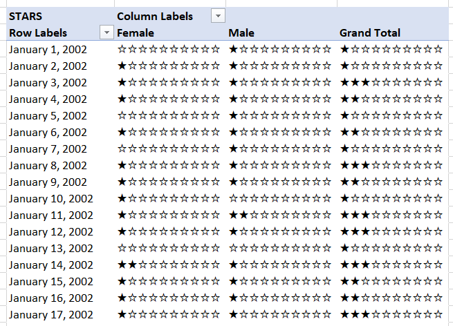
Let’s start off with recreating my ever-popular DAX star-ratings measure in MDX. Well, not exactly pure MDX, but did you know that in MDX you can call some Excel functions (in the same way you can call some VBA functions)? It’s a really, really bad thing to do from a query performance point of view, but it does allow you to do some useful calculations that might otherwise be impossible. Here’s a query on the Adventure Works cube that uses the Excel Rept() and Unichar() functions (functions that do not exist in MDX proper) to recreate my start-ratings measure:

[sourcecode language=”text” padlinenumbers=”true”]
WITH
MEMBER MEASURES.STARS AS
REPT(
UNICHAR(9733),
CINT([Measures].[Internet Sales Amount]/10000))
+
REPT(
UNICHAR(9734),
10-CINT([Measures].[Internet Sales Amount]/10000))

SELECT {[Measures].[Internet Sales Amount],MEASURES.STARS} ON 0,
ORDER(
[Date].[Date].[Date].MEMBERS,
[Measures].[Internet Sales Amount],
BDESC)
ON 1
FROM
[Adventure Works]
[/sourcecode]


image

Here’s the same measure used in a PivotTable:

image

SSAS Multidimensional: Are Your Indexes Processed?

If you are using SSAS Multidimensional and you use Process Update to process your dimensions, here’s something for you to try: run a Process Default on your cube. Does it finish in a few seconds? Then you’re ok. If it doesn’t, and it takes minutes or even longer then read on – you might have a problem that’s causing slow query performance.

One of the most common sources of query performance problems I see with my SSAS Multidimensional customers is unprocessed aggregations and indexes. If you run a Process Update on a dimension it may result in indexes and aggregations being dropped from partitions in your cubes; for more details on this, and why it happens, see this post:

https://blog.crossjoin.co.uk/2010/05/12/what-happens-when-you-do-a-process-update-on-a-dimension/

This classic post by Darren Gosbell explains how you can check if you have unprocessed aggregations on a partition:

http://geekswithblogs.net/darrengosbell/archive/2008/12/02/ssas-are-my-aggregations-processed.aspx

However, unprocessed indexes can also be a problem for query performance too. You can tell if the indexes on a partition are built by using the discover_partition_dimension_stat DMV. Here’s an example of how to use it for a partition in the Adventure Works database:

[sourcecode language=”text” padlinenumbers=”true”]
SELECT
DIMENSION_NAME, ATTRIBUTE_NAME, ATTRIBUTE_INDEXED,
ATTRIBUTE_COUNT_MIN, ATTRIBUTE_COUNT_MAX
FROM SystemRestrictSchema($system.discover_partition_dimension_stat
,DATABASE_NAME = ‘Adventure Works DW 2008’
,CUBE_NAME = ‘Adventure Works’
,MEASURE_GROUP_NAME = ‘Internet Sales’
,PARTITION_NAME = ‘Internet_Sales_2003’)
[/sourcecode]


[For some background on running SSAS DMV queries, see here]

Here’s what the above query returns, a list of dimensions and attributes that are related to the partition:

image

If the ATTRIBUTE_INDEXED column shows false then indexes are not built for the attribute on the dimension. In this example no indexes are built at all on the partition; if I do a Process Index or Process Default on this partition, here’s what the DMV returns:

image

Now you can see the ATTRIBUTE_INDEXED property is set to true for most attributes. Note that there is an (All) attribute that is never indexed, and if you have set the AttributeHierarchyEnabled property to false or the AttributeHierarchyOptimizedState property to NotOptimized on an attribute, it will not have indexes built for it either (this is typically done to improve processing performance – see here for a few more details).

In a real-world cube it is likely that only a few indexes will be dropped on partitions as a result of a Process Update on a dimension, and even then this will depend on whether any changes take place in the dimension’s data, so you will have to look down the list of attributes returned by this DMV very carefully to see if ATTRIBUTE_INDEXED returns false when it should be returning true.

The solution to this problem, as several of the posts I’ve linked to above suggest, is to always run a Process Default on your cube as the last step in your processing schedule. A Process Default will process any object that is in an unprocessed state, so it will automatically rebuild any aggregations or indexes that are dropped as a result of Process Updates on dimensions.

Power BI, SSAS Multidimensional And Dynamic Format Strings

If you’re building reports in Power BI against SSAS Multidimensional cubes then you may have encountered situations where the formatting on your measures disappears. For example, take a very simple SSAS Multidimensional cube with a single measure called Sales Amount whose FormatString property is set in SSDT to display values with a £ sign:

image

When you build a report using the Table visualisation in Power BI Desktop using this measure, the formatted values are displayed correctly:

image

However, if you add a SCOPE statement to the cube to alter the format string of the measure for certain cells, as in this example which sets the format string for the Sales Amount measure to $ for Bikes:

[sourcecode language=”text” padlinenumbers=”true”]
SCOPE([Measures].[Sales Amount], [Product].[Category].&[1]);
FORMAT_STRING(THIS)="$0,0.00";
END SCOPE;
[/sourcecode]

…then you’ll find that Power BI displays no formatting at all for the measure:

image

What’s more (and this is a bit strange) if you look at the DAX queries that are generated by Power BI to get data from the cube, they now request a new column to get the format string for the measure even though that format string isn’t used. Since it increases the amount of data returned by the query much larger, this extra column can have a negative impact on query performance if you’re bringing back large amounts of data.

There is no way of avoiding this problem at the moment, unfortunately. If you need to display formatted values in Power BI you will have to create a calculated measure that returns the value of your original measure, set the format string property on that calculated measure appropriately, and use that calculated measure in your Power BI reports instead:

[sourcecode language=”text”]
SCOPE([Measures].[Sales Amount], [Product].[Category].&[1]);
FORMAT_STRING(THIS)="$0,0.00";
END SCOPE;

CREATE MEMBER CURRENTCUBE.[Measures].[Test] AS
[Measures].[Sales Amount],
FORMAT_STRING="£0,0.00";
[/sourcecode]

image

Thanks to Kevin Jourdain for bringing this to my attention and telling me about the workaround, and also to Greg Galloway for confirming the workaround and providing extra details.

UPDATE October 2017: this issue appears to be fixed in the latest release of Power BI https://powerbi.microsoft.com/en-us/blog/power-bi-desktop-october-2017-feature-summary/#analytics