Finding All Selected Items In A Slicer In Excel 2016 Using TextJoin()

When you are using slicers with an Excel PivotTable it’s often useful to be able to get a comma-delimited list of the items selected in that slicer for use in a report title. It’s not easy to do though, and in fact this is one of those topics that lots of people have blogged about over the years: here’s my MDX approach, here’s Erik Svensen’s post on using the new DAX ConcatenateX() function, and there are also posts by Rob Collie like this one. None of these techniques are ideal though: my personal favourite is the ConcatenateX() approach, but that only works with SSAS Tabular 2016 (and then only if you can create a measure on the model) or Power Pivot in Excel 2016, and not at all if you’re using SSAS Multidimensional or earlier versions of SSAS Tabular.

However, after discovering the new TextJoin() function in Excel 2016 the other week I realised that this would provide yet another way to solve this problem. Here’s a simple example using a PivotTable and slicer connected to a Power Pivot model:

image

The highlighted cell F3 showing a comma-delimited list of all the items selected in the slicer has the following Excel formula:

[sourcecode language=”text” padlinenumbers=”true”]
=TEXTJOIN(
", ",
TRUE,
IFERROR(
CUBERANKEDMEMBER(
"ThisWorkbookDataModel",
Slicer_Product,
ROW(
INDIRECT("1:"&CUBESETCOUNT(Slicer_Product))
)
),
"")
)
[/sourcecode]

Important: this needs to be entered as an array formula, so instead of hitting Enter after typing in the formula you need to hit Ctrl+Shift+Enter. You’ll see the formula surrounded by braces {} in the formula bar when you do this:


image

image

This formula relies on the fact that the selection in a slicer (in the example above the slicer has the name Slicer_Product) can be treated the same as the output of the Excel CubeSet() function, which means that you can use the CubeSetCount() function to find the number of items selected and the CubeRankedMember() function to get the name of any single item in the selection. It also uses the Row()/Indirect() trick described here to create an array of numbers from 1 to the number of items selected in the slicer, which in turn provides the rank values to pass to the CubeRankedMember() function.

The beauty of this approach is that it works for Power Pivot and all versions of SSAS Tabular and Multidimensional, and doesn’t require any measures to be created on your models/cubes. It even works in Excel Online, so it will work inside Power BI, although it doesn’t seem to be possible to create array formulas in Excel Online yet so you need to create the formula on the desktop before you deploy. Of course you need the latest build of Excel 2016 for all this to work, and at the time of writing most people don’t have Excel 2016 and even if they do they probably won’t have a build (Version 16.0.6568.2025 or higher) with TextJoin() in it yet. But this will be a great solution in the distant future when everyone has Excel 2016, I promise!

You can download the sample Excel 2016 workbook here.

I also have to acknowledge the help of David Hager in writing this formula – we had a conversation about how TextJoin() behaves in array formulas in the comments of my earlier post and in doing so he provided the basic approach for me.

BI Survey 16

It’s that time of year again, so if you’ve got a few moments to spare here’s the link to take part in the BI Survey 16:

https://digiumenterprise.com/answer/?link=2908-SE68TH8Z

The BI Survey is the world’s largest survey of BI users and provides a fascinating insight into what’s really going on in the world of BI, as opposed to what the journalists and analysts are hyping.

In return for promoting it here, I get a free copy of the results and permission to blog about them. I’m particularly looking forward to finding out what it says about Power BI this year: just about all of the problems with the Excel/Power-add-ins combination identified in last year’s survey (data volume problems with 32-bit Excel, no real mobile story, the SharePoint dependency, confusion about what each of the add-ins does) have now been addressed with the new Power BI strategy, and I’m seeing a lot of customers starting projects with it.

Working With CSV Files That Contain Rogue Line Breaks In Power Query And Power BI

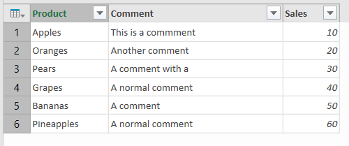
CSV files often contain text fields, and text fields often contain line breaks that shouldn’t be there (especially if the text is entered by end users). For example, here is are the contents of a simple CSV file that should contain three fields(Product, Comment and Sales) and six rows:

[sourcecode language=”text” padlinenumbers=”true”]
Product,Comment,Sales
Apples,This is a commment,10
Oranges,Another comment,20
Pears,A comment with a
line break in,30
Grapes,A normal comment,40
Bananas,A comment
with
two line breaks,50
Pineapples,A normal comment,60
[/sourcecode]

However, as you can see, the Comment field contains line breaks in some cases. If you try to load this file into Power Query/Power BI, you’ll see that it doesn’t handle things well:

image

The easiest way of solving this problem is to make sure you have double quotes around the text in the Comment field, so that Power Query/Power BI knows to ignore the line breaks:

[sourcecode language=”text” padlinenumbers=”true”]
Product,Comment,Sales
Apples,"This is a commment",10
Oranges,"Another comment",20
Pears,"A comment with a
line break in",30
Grapes,"A normal comment",40
Bananas,"A comment
with
two line breaks",50
Pineapples,"A normal comment",60
[/sourcecode]

image

[By the way, no text in the screenshot above has been truncated. The line breaks are still there in the Comment field; you can see the full text in the bottom pane of the Query Editor by clicking on a cell in the table.]

But what if you can’t fix the source data? I was asked this question the other week, and since I had been asked about it before and not come up with a good answer, I decided to spend some time researching the problem.

What I found was that it was relatively easy to write some M code that gave me the correct results, but very hard to write code that performed acceptably well on a large data set (I was testing on a CSV file containing almost half a million rows). Here’s the code for the function I ended up with:

[sourcecode language=”text” wraplines=”false” light=”true”]
(FileName as text, DelimiterCharacter as text, DelimitersPerLine as number, UseFirstRowAsHeaders as logical) =>
let
// Load file and buffer in memory
BufferedBinary = Binary.Buffer(File.Contents(FileName)),
// Convert to a single block of text
Source = Text.FromBinary(BufferedBinary),
// Find the position of all line breaks
LineBreaks = List.Buffer(Text.PositionOf(Source, "#(cr,lf)", Occurrence.All)),
// Get a list of numbers from 0 to the number of line breaks-1
LinePositions = List.Positions(LineBreaks),
// Count the number of line breaks
TotalLines = List.Count(LineBreaks),
// Split the text by line breaks
FirstSplit = Text.Split(Source, "#(cr,lf)"),
// On each line, count the number of column delimiter characters
DelimiterCounts = List.Buffer(
List.Transform(
LinePositions,
each List.Count(Text.PositionOf(FirstSplit{_},
DelimiterCharacter,
Occurrence.All)))),
// Loop through each line and
// a) Calculate a running total of the number of column delimiter characters on each line
// b) Divide the running total by the expected number of delimiters per line, and round down to the nearest integer
RunningSums = List.Buffer(
List.Generate(
()=>[Counter=0, RunningTotal=0],
each [Counter]<TotalLines,
each [Counter=[Counter]+1, RunningTotal=[RunningTotal]+DelimiterCounts{[Counter]}],
each Number.IntegerDivide([RunningTotal]+DelimiterCounts{[Counter]},DelimitersPerLine))),
// If the result of the division calculated in the previous step is
// the same as on the previous line, then the line break can be ignored
// so return null, otherwise return the position of the line break
FindFullLines = List.Transform(LinePositions, each if _=0 or RunningSums{_}<>RunningSums{_-1} then LineBreaks{_} else null),
// Remove nulls from the list
RemoveNulls = List.RemoveNulls(FindFullLines),
// Split the original text by the positions of the line breaks left
LineSplitterFunction = Splitter.SplitTextByPositions(List.Combine({{0},RemoveNulls})),
ActualLines = LineSplitterFunction(Source),
// Convert the result to a table
ConvertToTable = Table.FromList(ActualLines, Splitter.SplitTextByDelimiter(DelimiterCharacter), null, null, ExtraValues.Ignore),
// Use the first rows as headers if desired
PromoteHeaders = if UseFirstRowAsHeaders then Table.PromoteHeaders(ConvertToTable) else ConvertToTable
in
PromoteHeaders
[/sourcecode]

Assuming that you called this function LoadFile(), here’s an example of how to call it:

[sourcecode language=”text” padlinenumbers=”true”]
LoadFile(
//File name
"C:\MyFile.csv",
//Column delimiter character – in this case a comma
",",
//The expected number of commas to be found per line
//ie one less than the number of columns
2,
//If true then first row contains header values
true)
[/sourcecode]

The comments in the code should give you an idea of how it all works. A few other things to note:

  • If any of your lines contain extra columns, this approach won’t work
  • I’ve noticed a difference between how the Power BI Desktop and Excel 2016 behave with this code: the current Excel 2016 Query Editor will keep any line breaks after splitting on them, whereas Power BI Desktop does not. It’s easy to fix the Excel output though: just use the Clean transform to remove the line breaks.

I’m not really sure why it was so hard to come up with code that performed well, even after liberal use of List.Buffer(). It seemed like any time I referenced the original text (as returned by the Source step) in the List.Generate() function then performance died – so you’ll notice in the code above that I’m only referencing the list that contains the number of delimiters found per line.

Rendering Text On A Map With Power Query And Power Map

They say a good magician never reveals his tricks. Luckily, I’m a rubbish magician and so (at the request of Jason Thomas and David Eldersveld) I can reveal the secret behind one of the magic tricks I used in my sessions at SQLBits and the PASS Summit last year: my mind-reading card trick. More specifically, this post will show you how I was able to find out which card my helper had picked from a deck and how I was able to make its name appear in Power Map. Alas the video of the hour-long SQLBits session isn’t available for some reason, but the video of the shortened version of the session I did at the BI Power Hour at the PASS Summit is available for purchase here along with other, much more useful content.

First of all, the mind-reading bit. I hate to admit it but it had nothing to do with this rather fetching hat – the Microsoft Brain Interface – modelled here by Matt Masson:

image

In fact I had some accomplices (Bob Duffy and Carmel Gunn at SQLBits, Matt Masson at PASS) who entered the name of the card into a text file stored in OneDrive when my helper showed it to the audience. I then used the technique Melissa Coates blogged about here to read the name from the text file using Power Query on my laptop.

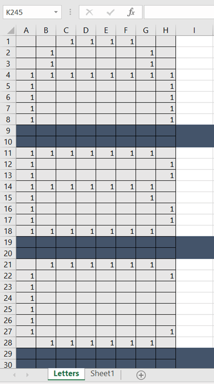
Second, the harder problem of taking the name of the card and making it appear in Power Map. Again, I used the magic of Power Query. On an Excel worksheet I used 1s and blanks to represent each letter of the alphabet in its own 8×8 grid:

image

…and then I read this into Power Query, matched each 8×8 grid up to the letter it represented, split the name of the card into letters, put the two together and got a table containing a set of data points that, when plotted on a custom map in Power Map, could be read as text:

image

You can download a modified version of the workbook here which reads data from the worksheet instead of a text file and renders the text over a regular map in Power Map. Here’s an example of the output:

Sadly I’m even less of an artist than I am a magician, and I admit that the output could be prettier. David Eldersveld recently showed off a very impressive Power BI report that uses a scatter chart to display the Power BI logo (you can see the report live here):

image

I guess the logical next step would be to take my code, move it to Power BI, add a column with date values in and use the play axis on the scatter chart to display animated text or pictures. But, to be honest, that might be too geeky a project even for me.

Disabling Excel PivotTable Grouping And Session Cubes In SSAS Multidimensional

The Excel PivotTable grouping functionality that is available when you are connected to an SSAS Multidimensional cube (but not a Tabular model) is a Very Bad Thing indeed. In my experience it is a major cause of query performance problems – not just for the person running the query, but because it is so resource intensive for everyone else trying to query the cube too. This post from a few years ago gives some more details about why custom grouping, and the CREATE SESSION CUBE MDX statements that it uses behind the scenes, are so expensive.

Up until now it was impossible to prevent users from using custom grouping but in a recent cumulative update this changed. First of all, I encourage you to read the details of the fix because you will probably want to install the relevant CU for security reasons anyway:

https://support.microsoft.com/en-us/kb/3080856

[And if you are wondering whether you should be installing CUs I strongly suggest you read this post by Aaron Bertrand]

Once the CU has been installed the following new property is added to the msmdrv.ini file:

\OLAP\Query\SessionCubesMode

This will be set to 1. Setting this property to 0 will prevent users from creating session cubes and therefore prevent them from using Excel’s custom grouping functionality.

My opinion is that it’s a good idea to disable session cubes and custom grouping even if you don’t know whether your users are using these features. Yes, your users will lose some functionality and some reports might even break, but you will also save yourself and your users a lot of problems. If your users need to do custom grouping in a report that is usually an indication that you have missed something in your dimension design, and that an extra attribute hierarchy or two is necessary.

[Thanks to Akshai for this information]

New Ways To Concatenate Text In Excel 2016 With CONCAT() And TEXTJOIN()

I don’t normally blog about Excel topics outside of Power Query and Power Pivot, but I think anyone who has ever done any serious work in Excel has found how difficult it is to concatenate more than two text values (although there are plenty of blog posts like this one showing how to do it). Well, not any more – Microsoft have finally got around to addressing this problem with two new Excel functions, TEXTJOIN() and CONCAT(). The announcement, plus news of other new Excel functions and a new funnel chart type, is here:

https://support.office.com/en-us/article/What-s-new-in-Excel-2016-for-Windows-5fdb9208-ff33-45b6-9e08-1f5cdb3a6c73

First, the bad news: at the time of writing you’ll only be able to use these functions in Excel on the desktop if you’re using the click-to-run version of Excel 2016 that you get through an Office 365 subscription (ie the version installed through the Office 365 portal that gets updated by Microsoft automatically – probably not the same version that you’re running on your desktop if you work for a big company). It is available in Excel Online and Excel Mobile too. I guess they’ll appear in the regular, Windows-installer version of Excel 2016 in a service pack at some point in the future.

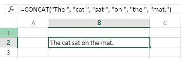
How about some examples? First of all, CONCAT() is a successor function for the old CONCATENATE() function – as far as I can see it does everything CONCATENATE() does but crucially also supports ranges as inputs as well as individual text values. So

=CONCAT("The ", "cat ", "sat ", "on ", "the ", "mat.")

Returns

The cat sat on the mat.

image

…but also, if you have each of your words in different cells (nb I’ve added spaces at the end of each word here), you can concatenate all the values in a range like this:

=CONCAT(B2:B7)

image

The TEXTJOIN() function is more flexible and I suspect will be very popular. It gives you two benefits over CONCAT():

  1. The ability to specify a delimiter – a character or characters (for example a comma or a space) to insert between each item of text you want to concatenate
  2. The ability to ignore empty values

Some examples…

First, using a space in the first parameter:

=TEXTJOIN(" ",FALSE,"The","cat","sat","on","the","mat.")

Returns once again

The cat sat on the mat.

…without having to add spaces to the end of each word, as I did with the CONCAT() example above:

image

And

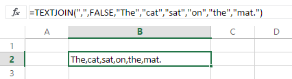
=TEXTJOIN(",",FALSE,"The","cat","sat","on","the","mat.")

Returns

The,cat,sat,on,the,mat.

image

Finally, here’s an example of how TEXTJOIN() can be used with a range with the second parameter being set to TRUE to ignore empty cells in a range:

=TEXTJOIN(",", TRUE,B2:B9)

With the data in the screenshot below again returns

The,cat,sat,on,the,mat.

image

You can see an Excel Online worksheet with all these examples here.

Analysing Power BI DMV Queries In Power BI Desktop

Experienced Analysis Services and Power Pivot developers will know all the interesting things you can learn from DMV queries. For example, in this blog post Kasper de Jonge shows how to use a DMV to find out which columns are using the most memory in a Power Pivot model; here’s an older post from me on using DMVs to show the dependencies between DAX calculations. There’s plenty of other interesting stuff about how data is stored and so on that you can find with a bit of digging, and there’s some reasonably up-to-date documentation on DMVs for SSAS here.

However, running DMV queries against a Power BI Desktop model (which of course runs a local version of the same engine that powers Analysis Services Tabular and Power Pivot) and more importantly doing something useful with the information they return, isn’t straightforward. You can run DMV queries from DAX Studio but that will only give you the table of data returned; you need to copy and paste that data out to another tool to be able to analyse this data. Instead it’s possible to use Power BI Desktop’s own functionality for connecting to Analysis Services to connect to its own local data model and run DMV queries.

If you’re connecting to an instance of Analysis Services in Power BI Desktop you need a server name and a database name and the same goes when you’re connecting Power BI Desktop to itself. This episode of Adam Saxton’s excellent Guy In A Cube YouTube show details how to connect SQL Server Profiler to Power BI Desktop in order to run a trace, and the method he uses to find the connection details also works for our purpose here; it’s definitely worth a watch because it goes into a lot of detail. However it’s much easier to get the connection details from DAX Studio using the following steps (thanks to Darren Gosbell for pointing this out):

  1. Open Power BI Desktop and load data as normal.
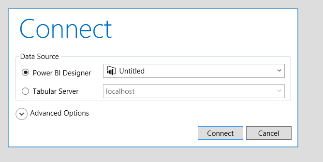
  2. Open DAX Studio and choose the Power BI Designer data source option:image
  3. Look in the bottom right-hand corner of the screen and you’ll see the server name, including the all-important port number, that you have connected to. In this case it’s
    localhost:52981image
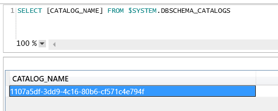
  4. Run the following DMV query in a DAX query window. This will give you the nasty GUID that is the name of the only database in the Power BI data model:

    [sourcecode language=”text” padlinenumbers=”true”]
    SELECT [CATALOG_NAME] FROM $SYSTEM.DBSCHEMA_CATALOGS
    [/sourcecode]

    image


  5. Now go back to Power BI Desktop, click the Get Data button and choose Analysis Services. In the connection dialog enter just the server name and port number and the database name found in the previous steps, as well as your DMV query:image


Once you have done this, you can load the results of your DMV query into the data model and analyse the results just like any other data. Here’s an M query using the DMV from the blog post by Kasper referenced earlier that looks at the memory used by just one table in the model:

[sourcecode language=”text”]
let
Source = AnalysisServices.Database(
"localhost:52981",
"1107a5df-3dd9-4c16-80b6-cf571c4e794f",
[Query="SELECT dimension_name, attribute_name, DataType,
(dictionary_size/1024) AS dictionary_size
FROM $system.DISCOVER_STORAGE_TABLE_COLUMNS"]),
#"Filtered Rows" = Table.SelectRows(Source,
each ([dimension_name] = "FactInternetSales"))
in
#"Filtered Rows"
[/sourcecode]

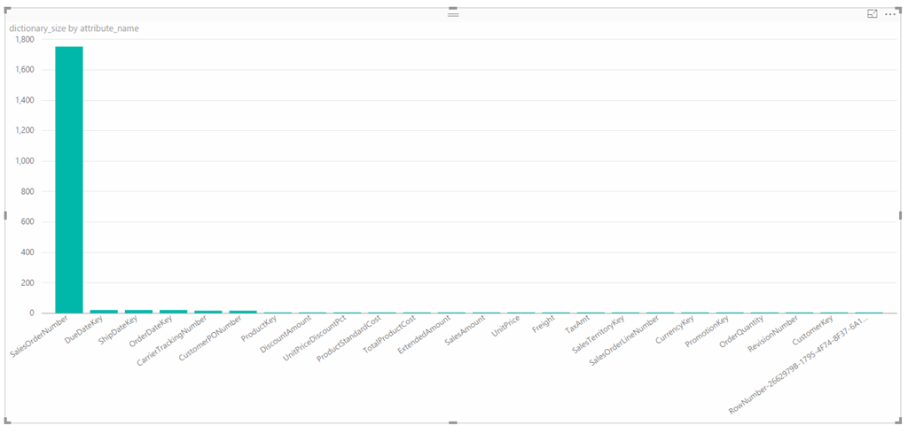
And here’s a bar chart built from that query showing clearly that the SalesOrderNumber column in the FactInternetSales table is very expensive:

image

Before you get too excited about this, there are two major problems you need to be aware of when using this technique:

  1. The port number used to connect to the local data model and the database name will change every time you open the Power BI Desktop file, so you will have to edit the connection information manually if you want to refresh the data after reopening.
  2. You won’t be able to make this connection refresh once you have published the file to PowerBI.com – so this will only work on the desktop.

That said, I think this is still very useful for development purposes. At some point I expect we’ll probably get a range of management reports in PowerBI.com that show similar data on published reports – just like we used to have in the old Office 365 Power BI.

Monitoring SSAS Multidimensional MDX Query Results Serialisation, Part 2

In part 1 of this series I looked at the basics of monitoring SSAS Multidimensional query resultset serialisation in Profiler. In this post, I’ll be taking a look at what happens for queries that return large amounts of data

Consider the following query on the Adventure Works DW database, which, when I run it in SQL Server Management Studio returns a cellset with 60391 rows:

[sourcecode language='text'  padlinenumbers='true']
SELECT
{[Measures].[Internet Order Quantity], 
[Measures].[Internet Sales Count]}
ON 0,
NON EMPTY
[Date].[Date].[Date].MEMBERS
*
[Customer].[Customer].[Customer].MEMBERS
*
[Product].[Product].[Product].MEMBERS
ON 1
FROM
[Adventure Works]
[/sourcecode]

image

There are a couple of interesting things to note about this query. First, SQL Server Management Studio on my laptop says that it takes nine seconds to run, even on a warm cache; the Duration column for the Query End event in Profiler, however, shows a value of around six seconds. The three second difference must be the time it takes for SSAS to return the cellset to SQL Server Management Studio, and for SQL Server Management Studio to render the results (my guess is that it’s the second operation that takes the majority of this time – other client tools may be more efficient at rendering large resultsets).

Secondly, in Profiler, you’ll see a much larger number of Serialize Results Current events. In situations where an axis contains more than a thousand tuples, or a cellset contains more than a thousand cells, you’ll see one Serialize Results Current event for each thousand tuples or cells. The ProgressTotal column will show values incrementing by one thousand up to the total number of tuples or cells. So, here’s some of what Profiler shows for the serialisation of the Rows axis:

image

…and here’s the end of the trace, showing the end of the serialisation of the cells (60391 rows * 2 columns = 120782 cells):

image

The third thing to notice is that there is only one Storage Engine operation – shown by the Query Subcube Verbose event in the first Profiler screenshot above – and that hits the Storage Engine cache and is so quick the Duration column shows 0 ms. Getting the raw data isn’t the problem here, and there aren’t any MDX calculations either – which means that it’s the Non Empty filter and construction of the cellset that is taking all the time. Since neither of these operations can be cached (although you can play tricks like this), this explains why the query always takes six seconds to run, even on a warm cache. Further investigation reveals that the Non Empty filter in fact only takes about a quarter of a second, so it’s the construction of a large cellset that’s the real problem here. This is why I say you should always avoid queries that return large amounts of data! SSAS is not very good at returning large resultsets.

Incidentally, don’t fall into the trap of thinking that the values shown in the Duration column for the Serialize Results End event only represents the amount of time taken to construct the cellset. It shows the amount of time since the Serialize Results Begin event, and in between the Begin and End events all kinds of other things necessary for the query to return (such as the evaluation of MDX calculations) could be going on. In a lot of cases the Serialize Results End event shows a duration that is almost the same as the duration for the whole query, but that only means that serialisation was able to start soon after the query began. In order to find the overhead of serialisation you need to work out how long all these other things take and subtract that from the duration shown for Serialize Results End, and that’s easier said than done.

Finally, what can you do to improve performance? Well, in the first post in this series I showed there was a tabular alternative to a cellset, and this is certainly a lot more efficient at returning large amounts of data (although you probably won’t have a choice in this unless you are building your own client tool, and, SSRS uses the tabular format anyway). For this query a tabular resultset is almost two seconds faster to return than a cellset, at just over four seconds:

image

There’s another important technique you can use, once that I have already mentioned in a blog post a couple of years ago but which is worth mentioning again: each cell returned by this query returns a large number of properties that you may not need, and these extra properties have a significant effect on the size of the resultset. Adding a CELL PROPERTIES clause to the query so that you only return the value property, like so:

[sourcecode language='text'  highlight='14']
SELECT
{[Measures].[Internet Order Quantity], 
[Measures].[Internet Sales Count]}
ON 0,
NON EMPTY
[Date].[Date].[Date].MEMBERS
*
[Customer].[Customer].[Customer].MEMBERS
*
[Product].[Product].[Product].MEMBERS
ON 1
FROM
[Adventure Works]
CELL PROPERTIES VALUE
[/sourcecode]

…takes another two seconds off the duration of the query, whether you use a tabular resultset or a cellset:

image

Monitoring SSAS Multidimensional MDX Query Results Serialisation, Part 1

Profiler (or indeed XEvents) can tell you a lot of interesting things about what happens when SSAS Multidimensional serialises the resultset returned by an MDX query. To be honest, this isn’t something I’ve looked at in detail before but recently I decided to do some research in this area – it turns out that monitoring the Profiler events related to serialisation can be very useful when you’re trying to understand what a Profiler trace is telling you about query execution as a whole.

To start off, let’s look at some very simple examples. Consider the following MDX query on the Adventure Works DW database:

[sourcecode language=”text” padlinenumbers=”true”]
SELECT
{[Measures].[Internet Order Quantity],
[Measures].[Internet Sales Count]}
ON 0,
[Date].[Calendar Year].[Calendar Year].MEMBERS
ON 1
FROM
[Adventure Works]
[/sourcecode]

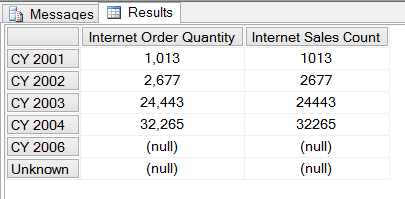
If you run it in SQL Server Management Studio in an MDX query window, you’ll get the following cellset back:

image

Running a Profiler trace using, amongst others, the Serialize Results Begin, Serialize Results Current and Serialize Results End events shows how SSAS is constructing the cellset returned:

image

The Serialize Results Begin event marks the point where SSAS starts to construct the cellset returned. The Serialize Results Current events that immediately follow it, with EventSubclass “1 – Serialize Axes” show SSAS serialising the tuples that are present on the Columns axis (listed as Axis 0 in the TextData column), the Rows axis (Axis 1) and the Where clause (Slicer Axis). The numeric values in the ProgressTotal column for the Serialize Results Current events shows the number of tuples on each axis: the two tuples on columns are the two measures, the six tuples on rows are the six years, and there’s one tuple on the slicer. After that SSAS gets the data for each of the cell values (as shown by the Query Subcube Verbose event – note that this query is running on a warm cache) and there is then a Serialize Results Current event with EventSubclass “2 – Serialize Cells”; the ProgressTotal column shows that twelve cells (2 columns * 6 rows) in total were returned.  The Serialize Results End event shows that SSAS has finished constructing the cellset and not surprisingly it’s followed immediately by the Query Cube End and Query End events.

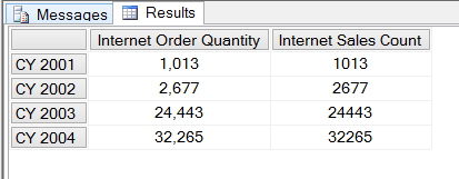
Sometimes SSAS needs to do a bit more work to find out what tuples are on an axis before serialisation can begin. The following query adds a NON EMPTY to the rows axis of the query above, so that only the rows that have values are returned:

[sourcecode language=”text” highlight=”5″]
SELECT
{[Measures].[Internet Order Quantity],
[Measures].[Internet Sales Count]}
ON 0,
NON EMPTY
[Date].[Calendar Year].[Calendar Year].MEMBERS
ON 1
FROM
[Adventure Works]
[/sourcecode]

image

In order to know which years will appear on rows it has to query the cube to find out which ones have values for the measures on columns; as a result the Profiler trace shows a Query Subcube Verbose event appearing now before Serialize Results Begin:

image

This trace deliberately doesn’t show any of events related to the NON EMPTY operation (something I’ll be writing about in future blog posts), but it looks like SSAS can work out which years have values and get the values needed for the cellset back in a single operation so there’s no need for another Query Subcube Verbose event before the Serialize Cells event. Note that now the empty rows have been excluded, the ProgressTotal shows that only four tuples are returned on rows and eight cells are returned overall.

Cellsets are not the only type of resultset that SSAS can return though. Some client tools, most notably Reporting Services, return a tabular dataset that doesn’t have the concept of axes; running the previous query in SSRS gives the following in Profiler:

image

As you can there is now only one Serialize Results Current event and it has the EventSubclass “3 – Serialize SQL Rowset” (even though this is still an MDX query); the ProgressTotal column shows four, which is the number of rows returned.

In Part 2, I’ll look at what happens when a query returns a much larger amount of data.

The Table.Schema() Function In Power BI/M

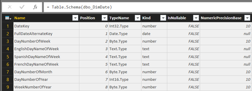
Yet another new M function for you this week: the Table.Schema() function, which returns information about the columns in a table. There’s some fairly detailed documentation about what it returns here; a simple demo is always a lot more helpful though, I think.

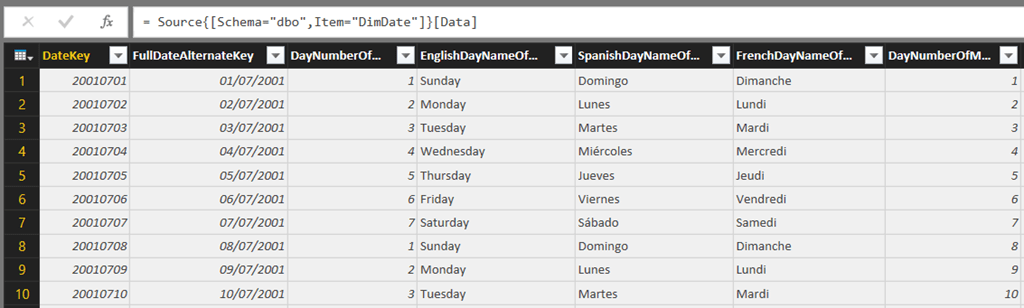
If you connect to the Adventure Works DW database in SQL Server and import the DimDate table, you’ll get an M query that returns the contents of that table (along with some extra columns that describe the relationships between that table and the others in the database):

[sourcecode language=”text” padlinenumbers=”true”]
let
Source = Sql.Database("localhost", "adventure works dw"),
dbo_DimDate = Source{[Schema="dbo",Item="DimDate"]}[Data]
in
dbo_DimDate
[/sourcecode]

image

If you add an extra step to this query that calls the Table.Schema() function on the table returned by the dbo_DimDate step, like so:

[sourcecode language=”text” highlight=”4″]
let
Source = Sql.Database("localhost", "adventure works dw"),
dbo_DimDate = Source{[Schema="dbo",Item="DimDate"]}[Data],
GetSchema = Table.Schema(dbo_DimDate)
in
GetSchema
[/sourcecode]

…you get a table with one row for each column in the table returned by dbo_DimDate, and a lot of columns that give you information on each column such as its position in the table, its M data type, its data type in the original data source and so on:

image

I can think of a lot of uses for this. Documenting a database is an obvious one; it would also serve as a much richer source of data when checking for changes in the structure of a data source, as I described here. Also, given how easy it is to tell whether two tables contain the same data in M, you could use this function to compare whether two tables have the same columns like so:

[sourcecode language=”text”]
let
Source = Sql.Database("localhost", "adventure works dw"),
dbo_DimDate = Source{[Schema="dbo",Item="DimDate"]}[Data],
SomeOtherTable =
Source{[Schema="dbo",Item="SomeOtherTable"]}[Data],
TablesEquivalent =
(Table.Schema(dbo_DimDate)=Table.Schema(SomeOtherTable ))
in
TablesEquivalent
[/sourcecode]

If you want more detail when doing comparisons you can do that with a little bit more M code, but that’s probably a topic for another post..