In the future you’re going see me writing blog posts on the official Power Query blog as well as here on my own personal blog, and indeed the first of these posts went live a few hours ago. It’s on a new M function called Table.StopFolding which, as the name suggests, stops query folding taking place:
I’m doing this a) because I was asked very nicely by the Power Query team if I could help out, and b) because it doesn’t make sense for announcements about new Power BI or Power Query functionality, however obscure, to be made on my own personal blog rather than on an official product blog. This isn’t going to affect the number of posts here though.
[Update May 2024 – the Power Query blog has now been taken down along with all of my posts there. I will republish the five posts I wrote here]
[This post was originally published on the Power Query blog which no longer exists. I have republished my posts from there here to make sure the content remains available.]
There’s a new aggregation option available for the Group By transformation in Power Query Online: percentiles. To see how it works, let’s see a simple example.
Consider the following Excel table containing information about invoices from different countries:
If you connect to this table from a Power BI or Power Platform dataflow, you can select the Country column and click the Group by button on the Transform tab in the ribbon:
When you do this the Group By dialog will open with the Country column selected in the Group by dropdown box. This is where you’ll see the new Percentile option in the Operation dropdown box; if you select it another box will appear underneath the Operation dropdown box where you can enter a number between 0 and 100 to indicate which percentile should be returned when the data is aggregated. You will also need to enter a new column name to contain the aggregated data and select a column containing the numeric data to be aggregated. Here’s what the Group By dialog would look like if you wanted to find the value for the 50th percentile from the Amount column for each country:
Click OK and here’s the output of the transformation:
This functionality uses the List.Percentile M function to do its work.
One last thing to mention is that if you’re using SQL Server or Azure Data Explorer as your data source query folding will take place for this transformation.
In it I showed how you could build a simple reporting solution using just Excel and Power Query, loading data into tables, handling parameterisation, making sure you get the best performance and so on. I think the session holds up pretty well: the functionality I showed hasn’t changed at all, and while in the meantime Power BI has reinvented itself and taken over the world I still think there’s a strong argument for using Excel plus Power Query instead of Power BI for some reporting scenarios (although it may be heresy to say so…).
If you follow the Excel blog you’ll know there have been a number of exciting announcements in the last few months, so I thought it would be interesting to take a look at some of them and consider the impact they have for BI and reporting use cases.
Power Query in Excel for the Mac
One of the priorities for the Excel Power Query team has been to get Power Query working in Excel on the Mac, and in the latest update we now have the Power Query Editor available. Data sources are still limited to files (CSV, Excel, XML, JSON), Excel tables/ranges, SharePoint, OData and SQL Server but they are some of the most popular sources. I’m not a Mac person so this doesn’t excite me much, but this does open up Power Query to a new demographic that has traditionally ignored Microsoft BI; for example, I was leafing through John Foreman’s excellent introductory data science book “Data Smart” recently and all the examples in it are in Excel to reach a mass audience, but… Excel for the Mac.
Power Query in Excel Online
This, on the other hand, is something I do care about: who cares what OS you’re running if you can do everything you need in the browser? Well now you can refresh Power Query in Excel Online, although again only a few data sources are supported at the moment: data in tables/ranges in the current workbook, or anonymous OData feeds. More data sources will be supported in the future and there will also be better integration with Office Scripts, so you’ll be able to refresh queries from Power Automate or via a button without needing VBA; you’ll also be able use the Power Query Editor in the browser too.
Before you get too excited about Power Query in Excel Online, though, remember one important difference between it and a Power BI report or a paginated report. In a Power BI report or a paginated report, when a user views a report, nothing they do – slicing, dicing, filtering etc – affects or is visible to any other users. With Power Query and Excel Online however you’re always working with a single copy of a document, so when one user refreshes a Power Query query and loads data into a workbook that change affects everyone. As a result, the kind of parameterised reports I show in my SQLBits presentation that work well in desktop Excel (because everyone can have their own copy of a workbook) could never work well in the browser, although I suppose Excel Online’s Sheet View feature offers a partial solution. Of course not all reports need this kind of interactivity and this does make collaboration and commenting on a report much easier; and when you’re collaborating on a report the Show Changes feature makes it easy to see who changed what.
More flexibility with Power Query data types
Being the kind of person who stores their data in Power BI I didn’t do much with Power Query data types when they were released; after all, you can create Organisation data types to access Power BI data from Excel and I prefer using Excel cube functions anyway. However if you’re not using Power BI then I can see how Power Query data types could be really useful for building reports that go beyond big, boring tables, making it much easier to create more complex report layouts.
Power Query connector for Power BI dataflows and Dataverse
Lastly, the feature I’m most excited about: the ability to load data from Power BI dataflows and Dataverse into Excel via Power Query. It’s not available yet although I promise it’s coming very soon! The ability to share cleaned and conformed data via dataflows direct to those Excel users who just want a data dump (rather than using Analyze in Excel on a Power BI dataset) will prove to be extremely popular, I think. There are a lot of improvements to dataflows coming soon too (you do remember to check the release notes regularly, don’t you?).
Conclusion
Overall it’s clear that Excel Power Query is getting better and better. It may never be able to keep pace with Power BI (what can?) but all these new features show that, for people who prefer to do everything in Excel, it’s making Excel a much better place to build reports. I feel like I need to update my SQLBits presentation now!
If you’re using DirectQuery mode in Power BI you may occasionally run into the following error message:
Couldn’t load the data for this visual
OLE DB or ODBC error: [Expression.Error] We couldn’t fold the expression to the data source. Please try a simpler expression..
What does it mean and how can you fix it?
To understand what’s going on here you must first understand what query folding is. There’s some great documentation here that I strongly recommend you read, but in a nutshell query folding refers to how the Power Query engine inside Power BI can push calculation and transformation logic back to whatever data source you’re using in the form of a query – for example a SQL query if your data source is a relational database. Most of the time when people talk about query folding they are using Import mode but it’s even more important in DirectQuery mode: in DirectQuery mode not only does every transformation you create in the Power Query Editor have to fold, but every DAX query (including all your DAX calculations) generated by the visuals on your report has to be folded into one or more queries against your data source too.
You can do some pretty complex things in the Power Query Editor and in DAX and the error message above is the error you get when Power BI admits defeat and says it can’t translate a DAX query generated by a visual on a report into a query against your data source. The cause is likely to be a combination of several of the of the following:
A complex data model
Complex DAX used in measures or calculated columns
The use of dynamic M parameters
Complex transformations created in the Power Query Editor
Unfortunately it’s hard to be more specific because Power BI can fold different transformations to different data sources and this error almost never occurs in simple scenarios.
How can you avoid it? Again, I can only offer general advice:
Don’t do any transformations in the Power Query Editor if you’re using DirectQuery mode. If you want to use DirectQuery you should always make sure your data is modelled appropriately in whatever data source you’re using before you start designing your dataset in Power BI.
Keep your data model as simple as possible. For example, avoiding bi-directional relationships is a good idea.
Try to implement as much of the logic for your calculations in your data source and reduce the amount of DAX you need to write.
Try to write your DAX in a different way in the hope that Power BI will be able to fold it.
A few months ago one of my colleagues at Microsoft, David Browne, showed me an interesting Power Query problem with how the Xml.Tables and Xml.Document M functions handle null or missing values. I’m posting the details here because the problem seems fairly common, it causes a lot of confusion and it’s not easy to deal with.
In XML there are two ways to represent a null or missing value:<a></a> or omitting the element completely. Unfortunately the Xml.Tables and Xml.Document M functions handle these inconsistently: they treat the <a></a> form as a table but the other as a scalar.
For example consider the following M query that takes some XML (with no missing values), passes it to Xml.Tables and then expands the columns:
Notice how code now contains scalar values but the value in that column on the second row is null.
You can probably guess the kind of problems this can cause: if your source XML sometimes contains missing values and sometimes doesn’t you can end up with errors if you try to expand a column that sometimes contains table values and sometimes doesn’t. It’s not a bug but sadly this is just one of those things which is now very difficult for the Power Query team to change.
There’s no easy way to work around this unless you can change the way your data source generates its XML, which is unlikely. Probably the best thing you can do is use the Xml.Document function; it has the same problem but it’s slightly easier to deal with given how it returns values in a single column, which means you can use a custom column to trap table values something like this:
 let
  Source
    = "<?xml version=""1.0"" encoding=""UTF-8""?>
    <Record>
     <Location>
        <id>123</id>
        <code>abc</code>
     </Location>
     <Location>
        <id>123</id>
        <code></code>
     </Location>
    <Location>
        <id>123</id>
        <code>124</code>
     </Location>
</Record>",
  t0 = Xml.Document(Source),
  Value = t0{0}[Value],
  #"Expanded Value"
    = Table.ExpandTableColumn(
    Value,
    "Value",
    {
      "Name",
      "Namespace",
      "Value",
      "Attributes"
    },
    {
      "Name.1",
      "Namespace.1",
      "Value.1",
      "Attributes.1"
    }
  ),
  #"Removed Other Columns"
    = Table.SelectColumns(
    #"Expanded Value",
    {"Name.1", "Value.1"}
  ),
  #"Added Custom" = Table.AddColumn(
    #"Removed Other Columns",
    "Custom",
    each
      if Value.Is([Value.1], type table) then
        null
      else
        [Value.1]
  )
in
  #"Added Custom"
[Thanks to David Browne for the examples and solutions, and to Curt Hagenlocher for confirming this is the way the Xml.Tables and Xml.Document functions are meant to behave]
[This post was originally published on the official Power Query blog, which has now been taken down. I’m republishing all my posts there to this blog to ensure the content remains available.]
Query folding is generally a good thing in Power Query: pushing transformations back to the data source means they almost always perform better. That’s not always the case though and sometimes you need to stop query folding taking place to improve performance. In the past there has been no easy way to do this: you could use the Table.Buffer M function but this also buffers an entire table into memory, which can lead to other, different performance problems; you could also add a transformation that you know doesn’t fold, such as adding an index column to your table, but again this could involve a performance penalty and what’s more if future versions of Power Query are able to fold the transformation then this approach will not work anymore. Now, however, there is a new M function called Table.StopFolding that is guaranteed to stop query folding taking place with no other side effects.
Here’s a simple example of how to use it. Consider the following M query which connects to SQL Server, gets data from the DimProductCategory table in the AdventureWorksDW2017 database and filters it so only the rows where the ProductCategoryKey column is greater than two are returned:
Here’s the SQL query generated by Power Query for this:
select [_].[ProductCategoryKey],
    [_].[ProductCategoryAlternateKey],
    [_].[EnglishProductCategoryName],
    [_].[SpanishProductCategoryName],
    [_].[FrenchProductCategoryName]
from [dbo].[DimProductCategory] as [_]
where [_].[ProductCategoryKey] > 2
As you can see, the filter has been folded and the WHERE clause of the SQL query contains the filter on ProductCategoryKey.
To stop query folding taking place for this filter transformation you can add an extra step to the M code of your query using the Table.StopFolding function like so:
The SQL query generated is now as follows, with no WHERE clause:
select [$Ordered].[ProductCategoryKey],
    [$Ordered].[ProductCategoryAlternateKey],
    [$Ordered].[EnglishProductCategoryName],
    [$Ordered].[SpanishProductCategoryName],
    [$Ordered].[FrenchProductCategoryName]
from [dbo].[DimProductCategory] as [$Ordered]
order by [$Ordered].[ProductCategoryKey]
The query result is still the same but the filter is not longer being folded back to SQL Server. Instead all the data is being returned to Power Query and the filter is taking place there.
I was looking at the output of Power Query’s Query Diagnostics feature recently (again) and trying to understand it better. One of the more confusing aspects of it is the way that the Power Query engine may evaluate a query more than once during a single refresh. This is documented in the note halfway down this page, which says:
Power Query might perform evaluations that you may not have directly triggered. Some of these evaluations are performed in order to retrieve metadata so we can best optimize our queries or to provide a better user experience (such as retrieving the list of distinct values within a column that are displayed in the Filter Rows experience). Others might be related to how a connector handles parallel evaluations.
I came up with the following M query to illustrate this:
#table(
    type table
    [#"Activity ID"=text],
    {{Diagnostics.ActivityId()}}
    )
If you paste this code into a new blank query:
…you have a query that returns a table containing a single cell containing the text value returned by the Diagnostics.ActivityId M function, which I blogged about here. The output – copied from the Data pane of the main Power BI window – looks like this:
The Diagnostics.ActivityId function is interesting because it returns an identifier for the currently-running query evaluation, so in the table above the value in the Activity ID column is the identifier for the query that returned that table.
If you run a Query Diagnostics trace when refreshing this query, you’ll see that the Activity Id column of the Diagnostics_Detailed trace query contains evaluation identifier values:
The following query takes the output of a Diagnostics_Detailed trace query and gets just the unique values from the Id and Activity Id columns:
let
    Source = #"Diagnostics_Detailed_2022-04-24_19:40",
    #"Removed Other Columns" = Table.SelectColumns(Source,{"Id", "Activity Id"}),
    #"Removed Duplicates" = Table.Distinct(#"Removed Other Columns")
in
    #"Removed Duplicates"
This makes it easy to see that my query was actually evaluated (or at least partially evaluated) three times when I clicked refresh. Since the value in the Activity Id column for Id 4.10 matches the value in the table loaded into my dataset, I know that that was the evaluation that loaded my table into the dataset.
In Power BI there’s a popular custom visual called “Filter by list” that lets you filter a Power BI report by any list of values that you paste into it. It can save you a lot of time in some scenarios, for example if you need to copy a list of values from another application and select those values in a slicer. In this post I’ll show how to recreate the same functionality in an Excel report connected to Power BI, Analysis Services or the Excel Data Model/Power Pivot using cube functions and dynamic arrays.
To show how I’m going to use a super-simple model built using Power Pivot consisting of the following single table:
The only other thing to note about the model is that it contains a measure called Sales Amount that sums up the values in the Sales column:
Sales Amount:=SUM(Sales[Sales])
Here’s what a PivotTable connected to this model looks like:
The aim here is to recreate this PivotTable using cube functions and allow the user to enter the list of invoice numbers used to slice the data either manually or by copy-and-pasting them into a table.
The first step is to create an Excel table (which I’ve called InvoiceNumbers) to hold the invoice numbers the user enters:
The next thing to do is to generate the text of the MDX set expression representing the list of invoice numbers in this table, which I’ve put in cell D2:
This text is used to create two named sets using the CUBESET function. The first, which I’ve put in cell D3, simply returns the set of invoice numbers that you get from evaluating the above MDX expression:
One last point: to keep things simple I’ve not included any error handling, which means that if a user enters a blank value or a value that isn’t an invoice number in the table the whole thing will break. To handle errors using the technique I blogged about here, alter the formula in D2 to:
I’ve said it before but I’ll say it again: I don’t publish book reviews here on my blog but I’m always happy to promote new Power BI books when they are published in return for a free copy.
Recently a friend and ex-Microsoft colleague of mine, Bhavik Merchant, published a book called “Microsoft Power BI Performance Best Practices” which I wrote the foreword for and I think (although of course I’m biased) it’s a good one. It’s about tuning all aspects of Power BI report and refresh performance, including DAX, data modelling, gateway configuration, Power Query/M and report design; it also covers the use of external tools like DAX Studio and Tabular Editor. From a purely technical point of view it gathers together a lot of useful information that is otherwise scattered across various documentation articles, blog posts, conference presentations and white papers; what I particularly liked, though, is the emphasis on methodology and how you should think about approaching performance tuning. If you’re new to Power BI this is a great resource but even experienced Power BI developers and consultants will learn something from it.
In the first post in this series I showed a simple example of how you can use the FORECAST.ETS function in Excel in combination with the Excel cube functions to do forecasting with Power BI data. In this post I’ll show you how you can:
Make the range of data that you display from Power BI, and pass into the FORECAST.ETS function, dynamic and controllable from a slicer
Make the number of periods that you forecast for dynamic too
Put both the actuals and forecast data together in a single range and display that in a chart
The first problem, making the range of data returned from Power BI via cube functions dynamic, is reasonably straightforward because it’s a variation on a technique I blogged about last year here. A slicer can be used to select the date range, which in turn can be captured using the CUBESET function, and finally the MAKEARRAY function can be used to return a dynamic array of dates and associated measure values. Here it is working:
Cell B2 contains the CUBESET formula that is used to capture the set of selected items in the slicer (which is called Slicer_Date):
=CUBESET("Price Paid", Slicer_Date, "Date Range Set")
B5 contains the dynamic array formula that returns the dates selected in the slicer using the CUBERANKEDMEMBER function:
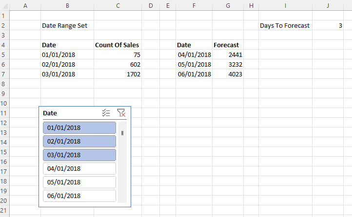
The second problem is how to create a similar dynamic range of forecast dates and values. Here’s the solution working:
J3 contains the number of days to forecast. F5 contains a formula that returns a list of dates whose length is controlled by the value in J3, and which starts the day after the last day in the range returned by the formula in B5. Here’s the formula in F5:
=SEQUENCE($J$2)+MAX(DATEVALUE($B$5#))
The formula in G5 returns the forecast values for the date range returned by F5, based on the values returned by the formulas in B5 and C5:
The third and final problem is how to combine these two ranges into a single range, like so:
The key to appending the Forecast values underneath the Count Of Sales values is the new VSTACK Excel function. So, for example, in I5 the following formula returns a dynamic array combining the dates used by the two ranges created above:
=VSTACK($B$5#, $F$5#)
For the Count Of Sales and Forecast columns I have padded the data out with zeroes, so for example the Count Of Sales column shows zeroes for the dates that contain forecast values and the Forecast column contains zeroes for the dates that contain Count Of Sales data. I did this by using VSTACK and appending/pre-pending an array containing zeroes created using MAKEARRAY. Here’s the formula for J5, ie the data in the Count Of Sales column:
=VSTACK($C$5#, MAKEARRAY($J$2, 1,LAMBDA(r,c,0)))
Here’s the formula for K5, ie the data in the Forecast column:
I could have used the HSTACK function to combine these three dynamic arrays into a single array but there’s no real benefit to doing this, and not doing it makes it easy to use the technique Jon Peltier describes here to display dynamic arrays in a chart. I won’t repeat what he says but you need to create Names for these last three dynamic arrays in order to be able to use them in a chart.
One last thing: I haven’t said anything about how to make sure the forecast values are useful and accurate. That’s because I’m not a data scientist and I don’t have any good advice to share. This is a very important topic, though, and I’m very grateful to Sandeep Pawar for providing some tips on Twitter here.